Oly Epigenetics
The reason the data looked terrible yesterday was because the polymer in the ABI hadn't been changed recently. Bruce did maintenance and re-ran the plate. I still had to run the modified size standard without the 250 and 340 peaks because they were still low quality. Size quality failed for samples DAB092_Msp1, DAB094_Msp1, FID093_MSp1. Added some new bins to the primer 1 panel and saved as primer 1.2.
FID094_Hpa1
April 1, 2013
Oly Epigenetics
Made a dilution plate (1:15) of the primer 1 select PCR and columns 1-5 of the primer 2 select PCR (see 3/29/13). Ran this plate on the ABI 3730 as described previously.
The size standards were not very good on this run for some reason (I used the ROX 500, same as last time, so I'm not sure what went wrong). Went through and corrected the incorrect size standard peaks. The size standard was good for the last time I ran samples, so I will use the locations of these previous peaks to call the correct peaks this time (used data from 3/25/13).
| Size Standard |
Peak Location 3/25 |
| 35 |
942 |
| 50 |
1080 |
| 75 |
1370 |
| 100 |
1640 |
| 139 |
2090 |
| 150 |
2202 |
| 160 |
2315 |
| 200 |
2787 |
| 250 |
3355 |
| 300 |
3995 |
| 340 |
4470 |
| 350 |
4593 |
| 400 |
5230 |
| 450 |
5813 |
| 490 |
6298 |
| 500 |
6397 |
The MSAFLP data looks really bad too, so something went wrong.
I also looked at the data from primer set 2. The size standard also looks bad, especially at peaks 35, 250, 340, and >400. The MSAFLP peaks are also unreadable.
March 29, 2013
Oly Epigenetics
Select fluorescent PCR using primer pair 1 of all samples except for CAS.001-008, which were previously analyzed (see 3/25/13). This same plate layout will be used for all other primer pairs.
Also did fluorescent PCR for primer set 2.
March 28, 2013
Oly Epigenetics
Made panels for primer sets 3, 4, and 5. In primer 5, the size standard peak for sample CAS002 at 150 bp is sloppy, but still called correctly. The same blobby peak shows up in the FAM dye in this sample.
March 27, 2013
Oly Epigenetics
Fragment analysis using GeneMapper. Ran analysis in software of all samples using the primer 1 ETS method. Size standard peaks were called correctly in all samples (off-size peak in beginning - primer dimer - was not called). The size standard peaks all overlay on top of each other. It also appears that all fragment peaks are well within the size limit (500 bp) of the standard.
4 of the samples have peaks that are slightly broader than accepted by the quality standards: CAS.002 Msp5, CAS.001 Msp 3, CAS.002 Msp4, CAS.002 Msp7.
Samples resulting from different primers really need to be analyzed separately otherwise there are too many bins.
For primer 1:
Manually removed and added bins so that only probable peaks are called.
Deleted allele calls that were of peaks that are either very very small and most likely not real or "shoulders" of real peaks (preceded real peaks).
This entire process is creating a panel of bins to streamline future analysis of fragments for this primer set. The panel is called "primer 1 0325". The other primer panels will similarly be named. Panel for primer 2 is also completed.
March 25, 2013
Oly Epigenetics
Did fragment analysis on PCR done 3/21/13. Diluted the PCR product 1:15 in water. Put 5 µl of 500 rox size standard in 745 µl formamide and aliquoted 15 µl to each well in a plate (odd columns only since this is only 1 run), then added 1 µl of diluted PCR product. Ran plate on ABI 3730 xl.
March 21, 2013
Oly Epigenetics
Learning Genemapper
The manual for AFLP analysis in Genemapper can be found here: http://www.icmb.utexas.edu/core/DNA/Information_Sheets/Genotype/GeneMapper_AFLP_Guide.PDF
My tutorial with the Genemapper example data is called "AFLP Tutorial2".
Began analyzing my own data from PCR plate 1. Imported all data from primer pair 1. Analysis Method is called "primer 1 ETS". I basically followed the tutorial instructions except for some changes, which I will include. in the analysis method editor, allele tab, analysis range is 50-1000 bp. Also in allele tab, chose "name alleles using bin names".
DAB.093, which didn't amplify on 3/1/13, did not show any peaks.
Incorrect size standard peak of 47 called on primer peak at ~1477. Followed instructions on p. 47 of manual to get rid of it. Re-analysis of the data after this got rid of all the yellow triangles in the OS column. All of the SQ column is still red, however (poor quality). This means that the size calling based on the standard (created custom standard called ROX 1000 with correct peak sizes for this standard) is of low quality. This seems to be because the size standard peaks are double peaks. I went through and made sure that the standard was caused for the first peak in the double for each one. Also, deleted the label for peak 946 because that is not within the range of the data.
None of this work, the ROX 1000 is kind of crap. I'm going to PCR 8 samples for all 6 of my primer pairs and run them with 500 ROX.
Did fluorescent select PCR of 8 samples for each of the 6 primer pairs (1,2,3,4,5,7). NB: regular amplitaq was used for primer pair 1, amplitaq gold was used for the rest. PCR layout is here: https://www.evernote.com/shard/s242/sh/da6fba3d-32bc-4828-9778-64507a8a74c0/bba0926cf39aecef5ed3637aa66b048e
March 15, 2013
Secondary Stress: Proteomics
Conservation Physiology revisions
Did revigo analysis on DAVID done yesterday. The resulting list is very small, so limited it to tiny (allow similarities no greater than 0.4).
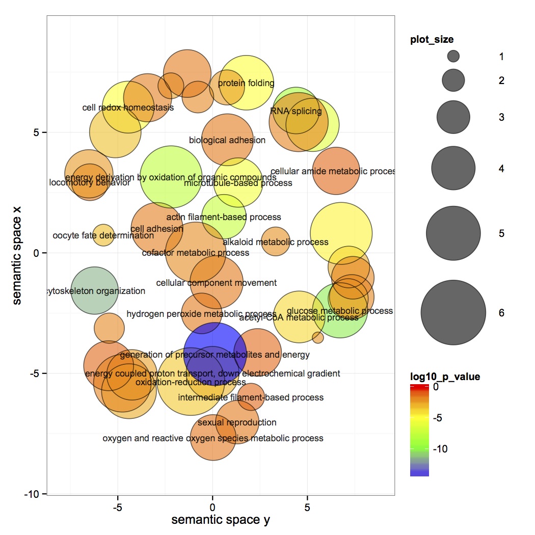
Joined enriched GO terms from DAVID with GO Slim terms.
SELECT * FROM [sr320@washington.edu].[ETS_Enriched_DAVID_GO]
LEFT JOIN [sr320@washington.edu].[GO_to_GOslim]
ON [sr320@washington.edu].[ETS_Enriched_DAVID_GO].Number=[sr320@washington.edu].[GO_to_GOslim].[GO_id]
Joined the newly filtered protein list (n=1044) with NSAF values with GO and GO Slim terms.
SELECT * FROM [sr320@washington.edu].[ETS_NSAF_oysters]
LEFT JOIN [dhalperi@washington.edu].[SPID_GOnumber.txt]
ON [sr320@washington.edu].[ETS_NSAF_oysters].SPID=[dhalperi@washington.edu].[SPID_GOnumber.txt].A0A000
SELECT * FROM [Cgigas proteins NSAF with GO]
LEFT JOIN [sr320@washington.edu].[GO_to_GOslim]
ON [Cgigas proteins NSAF with GO].[GO:0003824]=[sr320@washington.edu].[GO_to_GOslim].[GO_id]
Also made a histogram of the frequency of log(NSAF) (where nsaf = for total spec counts across all samples) and the distribution was normal.
March 14, 2013
Secondary Stress: Proteomics
Conservation Physiology revisions
To be included in analyses, each protein must have at least 2 unique peptide hits (in a single technical replicate) and at least 4 total spectral counts across all replicates. This ends up being 1044 proteins. For each oyster (total spec counts summed across technical replicates), calculated NSAF: (SpC/L)/(sum of all SpC/L for that oyster), where SpC = spectral count and L = protein length. Made plots of correlations between each oyster so that log(NSAF) of oyster A is plotted against log(NSAF) of oyster B for each protein for all 6 comparisons. Calculated R^2 values for the correlations with rSquared in R. Also plotted the 1:1 line in magenta on each of the correlation plots.
DAVID (v 6.7) analysis of enriched proteins in the gill tissue. Background proteome = Cg proteome db evalue -10, gene list = proteins that passed filters mentioned above. Results from GO BP FAT show 263 enriched GO terms in gill vs. entire proteome.
March 12, 2013
Secondary Stress: Proteomics
Joined files created 2/28 and 3/7 (Skyline results with peptides that match uniquely to a protein and only top 3 abundant peptides per protein for high and low pCO2) each to KEGG blast results.
SELECT * FROM [table_high pco2 for ipath.txt]
LEFT JOIN [table_Cgigas_proteomev9_kegg_match]
ON [table_high pco2 for ipath.txt].Protein=[table_Cgigas_proteomev9_kegg_match].Column1
Averaged expression values across oysters within each treatment. Joined together files of protein ID, peptide sequence, average expression, and KEGG ID for low and high pCO2.
SELECT * FROM [table_high pco2 avg exp. txt]
LEFT JOIN [table_low pco2 avg exp.txt]
ON [table_high pco2 avg exp. txt].Peptide=[table_low pco2 avg exp.txt].Peptide
Then did left join of high to low pco2 (opposite order as above) to get a list of the peptides from the low pco2 list that did not match to any in the high pco2.
Averaged peptide expression within each protein so now there is one expression value for each protein. Joined this SQL table to a table of the CGI IDs from high and low pCO2 joined to KEGG IDs.
SELECT Protein, avg(AvgExpHigh), avg(AvgExpLow) FROM [table_Combined pCO2 avg exp.txt]
Group by Protein
SELECT * FROM [Skyline high and low pCO2 avgd by protein]
LEFT JOIN [table_Combined pCO2 avg exp with Kegg.txt]
ON [Skyline high and low pCO2 avgd by protein].Protein=[table_Combined pCO2 avg exp with Kegg.txt].Protein
The pathway components in red show the proteins that are identified in the dataset.
https://www.evernote.com/shard/s242/sh/b59a5540-9104-4cb3-a773-bdd48874854c/4f93f4e691036d065e332c461abc6547
The pathway components in purple show components that are expressed more at low pCO2, those in green are expressed more at high pCO2. The input file for this is called ipath input 1.
https://www.evernote.com/shard/s242/sh/98249a09-9873-4405-9d14-ca0edeb8e60a/9d84d6b9889cd5ad1ea297038db3cf23
Oly Epigenetics
Prepared dilution plate (1:15) of PCR plate 1 done on 3/1/13. Diluted 10 µl of ROX 1000 in 1490 µl Formamide. Aliquoted 15 µl of the formamide-ROX into sequencing plate and added 1 µl of diluted PCR product to each well. Did fragment analysis on ABI 3730xl.
March 8, 2013
Secondary Stress: Proteomics
Revisions of Conservation Physiology paper
For all low pCO2 (no MS) oysters, made new files with one column of protein ID, one column of unique peptide hits, and 1 column of total spectral count. Combined all the unique protein identifications across these files into a file of all proteins sequenced.
March 7, 2013
Secondary Stress: Proteomics
For peptides with Skyline expression values for the low pCO2 oysters, created a file similar to that created for high pCO2 2/28/13. Removed peptides that mapped to multiple proteins. Peak areas for technical replicates were averaged for each oyster. Based on the total peak area across all biological and technical replicates, retained only the 3 most abundant peptides for each protein.
Checked on the status of the KEGG blast - about 15,000 matches have been made so it is just over halfway done.
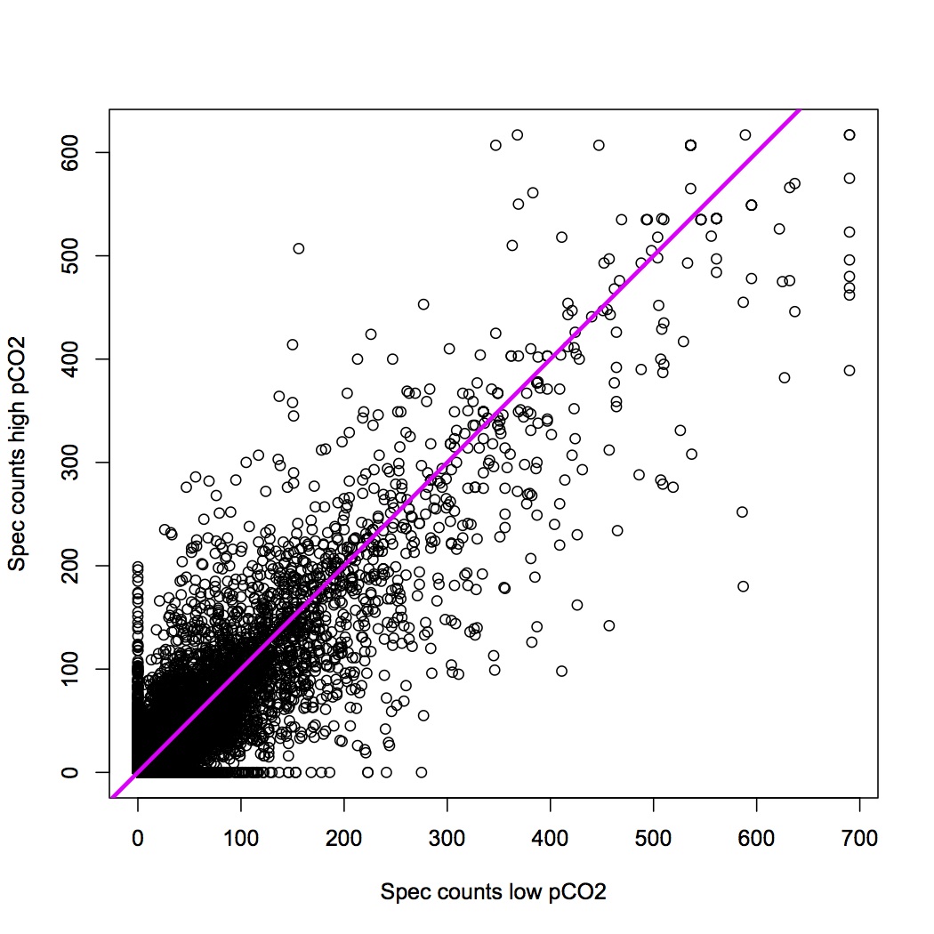
To further investigate correlations between spectral counts, uploaded files of spec counts per peptide for all low and all high pCO2 oysters to SQL and joined to a "backbone" of all unique peptides across all 8 samples.
SELECT [table_peptide IDs for low and high pco2.txt].*,[table_101B2_01_speccounts.txt].*,[table_101B2_02_speccounts.txt].*, [table_101B2_03_speccounts.txt].*, [table_101B5_01_speccounts.txt].*, [table_101B5_02_speccounts.txt].*, [table_101B5_03_speccounts.txt].*, [table_101B8_01_speccounts.txt].*, [table_101B8_02_speccounts.txt].*, [table_101B8_03_speccounts.txt].*, [table_101B11_01_speccounts.txt].*, [table_101B11_02_speccounts.txt].*, [table_101B11_03_speccounts.txt].*, [table_103B221_01_speccounts.txt].*, [table_103B221_02_speccounts.txt].*, [table_103B221_03_speccounts.txt].*, [table_103B224_01_speccounts.txt].*, [table_103B224_02_speccounts.txt].*, [table_103B224_03_speccounts.txt].*, [table_103B227_01_speccounts.txt].*, [table_103B227_02_speccounts.txt].*, [table_103B227_03_speccounts.txt].*, [table_103B230_01_speccounts.txt].*, [table_103B230_02_speccounts.txt].*, [table_103B230_03_speccounts.txt].*
FROM [table_peptide IDs for low and high pco2.txt]
LEFT JOIN [table_101B2_01_speccounts.txt]
ON [table_101B2_01_speccounts.txt].ProtPep=[table_peptide IDs for low and high pco2.txt].Column1
LEFT JOIN [table_101B2_02_speccounts.txt]
ON [table_101B2_02_speccounts.txt].ProtPep=[table_peptide IDs for low and high pco2.txt].Column1
LEFT JOIN [table_101B2_03_speccounts.txt]
ON [table_101B2_03_speccounts.txt].ProtPep=[table_peptide IDs for low and high pco2.txt].Column1
LEFT JOIN [table_101B5_01_speccounts.txt]
ON [table_101B5_01_speccounts.txt].ProtPep=[table_peptide IDs for low and high pco2.txt].Column1
LEFT JOIN [table_101B5_02_speccounts.txt]
ON [table_101B5_02_speccounts.txt].ProtPep=[table_peptide IDs for low and high pco2.txt].Column1
LEFT JOIN [table_101B5_03_speccounts.txt]
ON [table_101B5_03_speccounts.txt].ProtPep=[table_peptide IDs for low and high pco2.txt].Column1
LEFT JOIN [table_101B8_01_speccounts.txt]
ON [table_101B8_01_speccounts.txt].ProtPep=[table_peptide IDs for low and high pco2.txt].Column1
LEFT JOIN [table_101B8_02_speccounts.txt]
ON [table_101B8_02_speccounts.txt].ProtPep=[table_peptide IDs for low and high pco2.txt].Column1
LEFT JOIN [table_101B8_03_speccounts.txt]
ON [table_101B8_03_speccounts.txt].ProtPep=[table_peptide IDs for low and high pco2.txt].Column1
LEFT JOIN [table_101B11_01_speccounts.txt]
ON [table_101B11_01_speccounts.txt].ProtPep=[table_peptide IDs for low and high pco2.txt].Column1
LEFT JOIN [table_101B11_02_speccounts.txt]
ON [table_101B11_02_speccounts.txt].ProtPep=[table_peptide IDs for low and high pco2.txt].Column1
LEFT JOIN [table_101B11_03_speccounts.txt]
ON [table_101B11_03_speccounts.txt].ProtPep=[table_peptide IDs for low and high pco2.txt].Column1
LEFT JOIN [table_103B221_01_speccounts.txt]
ON [table_103B221_01_speccounts.txt].ProtPep=[table_peptide IDs for low and high pco2.txt].Column1
LEFT JOIN [table_103B221_02_speccounts.txt]
ON [table_103B221_02_speccounts.txt].ProtPep=[table_peptide IDs for low and high pco2.txt].Column1
LEFT JOIN [table_103B221_03_speccounts.txt]
ON [table_103B221_03_speccounts.txt].ProtPep=[table_peptide IDs for low and high pco2.txt].Column1
LEFT JOIN [table_103B224_01_speccounts.txt]
ON [table_103B224_01_speccounts.txt].ProtPep=[table_peptide IDs for low and high pco2.txt].Column1
LEFT JOIN [table_103B224_02_speccounts.txt]
ON [table_103B224_02_speccounts.txt].ProtPep=[table_peptide IDs for low and high pco2.txt].Column1
LEFT JOIN [table_103B224_03_speccounts.txt]
ON [table_103B224_03_speccounts.txt].ProtPep=[table_peptide IDs for low and high pco2.txt].Column1
LEFT JOIN [table_103B227_01_speccounts.txt]
ON [table_103B227_01_speccounts.txt].ProtPep=[table_peptide IDs for low and high pco2.txt].Column1
LEFT JOIN [table_103B227_02_speccounts.txt]
ON [table_103B227_02_speccounts.txt].ProtPep=[table_peptide IDs for low and high pco2.txt].Column1
LEFT JOIN [table_103B227_03_speccounts.txt]
ON [table_103B227_03_speccounts.txt].ProtPep=[table_peptide IDs for low and high pco2.txt].Column1
LEFT JOIN [table_103B230_01_speccounts.txt]
ON [table_103B230_01_speccounts.txt].ProtPep=[table_peptide IDs for low and high pco2.txt].Column1
LEFT JOIN [table_103B230_02_speccounts.txt]
ON [table_103B230_02_speccounts.txt].ProtPep=[table_peptide IDs for low and high pco2.txt].Column1
LEFT JOIN [table_103B230_03_speccounts.txt]
ON [table_103B230_03_speccounts.txt].ProtPep=[table_peptide IDs for low and high pco2.txt].Column1
Graph of correlation (each dot represents a peptide) of sums of spec counts for high and low pCO2. The pink line is the 1:1 line.
March 5, 2013
Bioinformatics: Assignment 8
Converted vcf file to gff in iPlant (VCG to GFF3). Uploaded to galaxy and viewed using trackster against the C. gigas genome. this results in an error, so I am visualizing in igv.
https://www.evernote.com/shard/s242/sh/48c52c8f-20ff-4f48-b06c-2fa80c96b331/fb9850f68bde673132e703385a5f27f2
Converted GFF To a BED file in galaxy and viewed the SNPs using circster: https://www.evernote.com/shard/s242/sh/1447ebee-81d5-4c30-b90b-1043c9a5d7d6/a05c491eef8c4fd7d77b2c6d9debe404. I also viewed in trackster (name = SNPs).
Secondary Stress: Proteomics
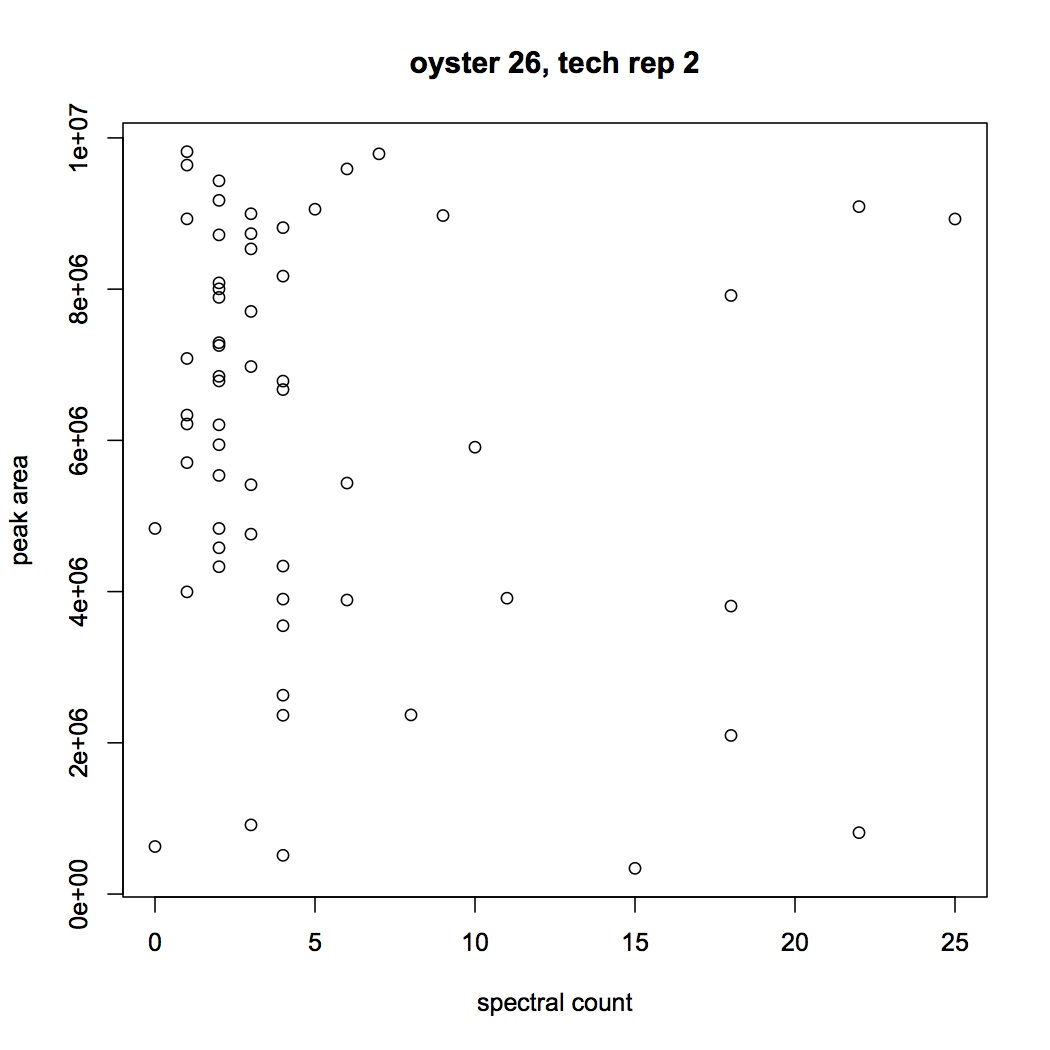
I'm trying to see if there is a correlation between spectral counts and peak area (Skyline) for the peptides. In SQL share I joined together peak area and spec count data for each peptide (I've done this for oyster 101B2 tech rep 1, 101B2_01, and 101B26_02). It does not look like there is anything approximating a linear correlation between the 2 expression statistics.
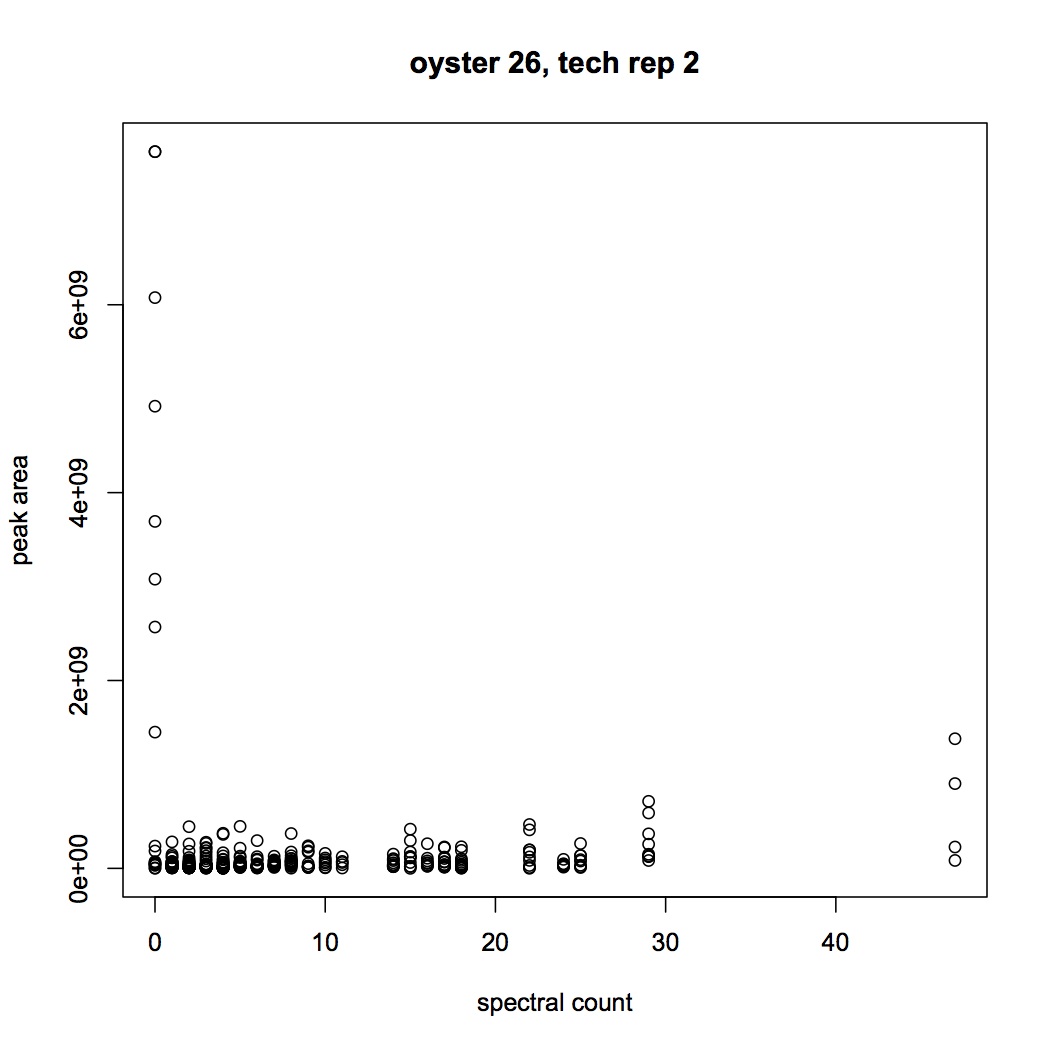
Did the same graph but with a cutoff of E6 for the peak areas.
Associating C. gigas proteins with KEGG IDs. Downloaded KEGG ID sequences (see 2/28/13) and made a blast db.
./makeblastdb -in /Users/Emma/Documents/kegg/KEGG_IDs.txt -dbtype prot -out /Users/Emma/Documents/kegg/kegg_db_030513
blastp of oyster proteome (from genome project) against KEGG db.
./blastp -num_threads 8 -out /Users/Emma/Documents/kegg/Cgigas_proteomev9_kegg_match -db /Users/Emma/Documents/kegg/kegg_db_030513 -outfmt 6 -evalue 1E-5 -max_target_seqs 1 -query /Volumes/web/oyster/oyster_v9_aa_format1.fasta
March 4, 2013
Secondary Stress: Fatty acids
I met with Mike Brett this morning to discuss my results. He says the analysis so far looks good and there's really tight replication across samples so he thinks the data are good overall. He suggested that I look at total lipids per dry weight for the oysters to see if there is a difference in overall fat content.
Oly Epigenetics
Made a dilution plate to run a dilution test of the fluorescent select PCR done 3/1/13. Used columns 2 and 6 from the PCR plate and diluted each of these 1:10, 1:20, 1:50 in nanopure water (this is 6 columns, 48 samples, equal to one run on the 3730xl). I mixed 5 µl ROX1000 size standard with 745 µl formamide and aliquoted 15 µl of this into each well for sequencing. Then added 1 µl of PCR product to the formamide/ROX mixture. Plate was run with a long run on the 3730 xl. It looks like somewhere between then 1:10 and 1:20 dilutions will work best. Identified the size peaks in the ROX1000 (https://www.evernote.com/shard/s242/sh/d54bd104-56f7-47ae-98d4-ad10cf23f643/2cc6cf532fa88f13b3058805f7a03c82). I had stored the ROX at -20°C because it arrived on ice, but it should be stored at 4°C (it has been moved to the fridge).
Bioinformatics: Assignment 8
Can't figure out how to use the SNP output from 2/28/13. Mac says that SR said to use Find SNPs - mpileup in iPlant. Used C. gigas genome as reference and RNASeq output accepted hits.bam as the bam file. First 26 lines of file need to be removed, however galaxy isn't working right now...
Secondary Stress: Proteomics
Worked with Brendan to figure out why Skyline can't upload all the raw files at once. I was able to upload ~70% of the raw files. Brendan figured out that one of the reasons why all the peptides weren't registering in the library was because the instrument max in the transition settings needs to be at 2,000.
March 1, 2013
Oly Epigenetics
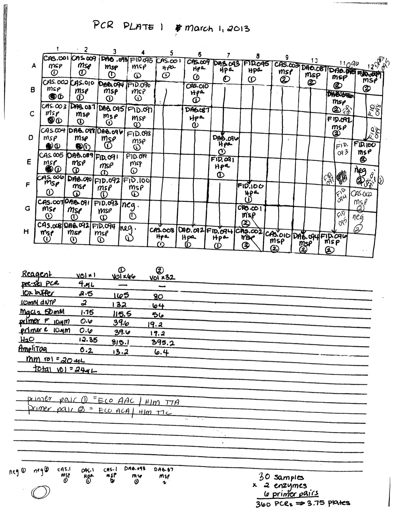
Select PCR with fluorescent primers. I am using only the DAB.091 sample extracted 2/8/13. PCR reaction was prepared as follows for Msp and Hpa for primer pair 1 and Msp only for primer pair 2: 4 µl pre-select PCR product, 2.5 µl 10X amplitaq buffer (no salt), 2 µl 10 mM dNTPs, 1.75 µl 50 mM MgCl2, 0.6 µl of each 10 µM primer (Eco primer is fluorescent), 12.35 µL H2O, 0.2 µl amplitaq. Total reaction volume = 24 µl. PCR was run on thermalcycler protocol PRESEL (see 2/12/13). New primer working stocks were made for H/M select primers TCG and TGC.
3 µl of PCR product was mixed with 5 µl loading dye and run for 30 minutes on a 1% agarose gel with EtBr at 100 V. Both primer pairs amplified product on the gel and there was no contamination in the negative controls. One sample (DAB.093) did not amplify.
https://www.evernote.com/shard/s242/sh/261907da-76e6-4372-ad30-5f57e20667a4/7e4679b8ab89bfd85430f53c43e8c87b
Secondary Stress: Proteomics
Brendan helped me with Skyline to see if we can get it to analyze all proteins instead of the pre-selected 357. We still used the oyster proteins library previously created. The protein/peptide tree was populated with the entire C. gigas proteome (from the version 9 sequencing project). Peptides that did not match those in the library were removed. Also removed from the peptide tree were duplicate peptides (peptides that matched to more than one protein) and empty proteins. Raw file results were imported as single injections.
February 28, 2013
Bioinformatics: Assignment 8
Set up user account on iPlant. Uploaded RNA-Seq files for 3' RNA-Seq of C. gigas exposed to OA (sequenced by Eli).
Also uploaded oyster genome v9. Chose Tophat to map RNA-Seq files to genome. Settings: FASTQ quality scale = illumina 1.9 (PHRED33), anchor length = 8, max number of mismatches = 2, min intron length = 70, max intron length = 50000, min isoform fraction = 0.15, max # alignments = 20, min intron length during split-segment = 50, max intron length during split-segment = 50000,# mismatches for reads mapped independently = 2, min length read segments = 20. top hat version 1.4.1, bowtie version 0.12.7.
Secondary Stress: Proteomics
To use iPath protein/peptide IDs need to be associated with either COG or KEGG IDs. This can be done in batches on the uniprot website (ID mapping). Steven also has a file of protein sequences corresponding to KEGG IDs which could be used as a db in a pblast. (http://eagle.fish.washington.edu/trilobite/KEGG/release/current/seq_pep/genes)
Took high pCO2 Skyline output from 12/11/12 and edited it to fit specifications of good analysis of skyline data: got rid of peptides mapping to multiple proteins and only kept top 3 abundant peptides for each protein. First got rid of all peptides with charge state > 2. Then created one column of peak areas for each oyster (technical replicates separate). Made a pivot table of the peptide sequences (count total) - there should only be 3 per peptide (peptides should not show up more than 1 time per technical replicate). Anything with a count > 3 was removed from the data set (~20 peptides). File = Skyline high pCO2 022813. In SQL share averaged peptide peak areas across technical replicates for each oyster.
Select ProtPep, avg(oyster11), avg(oyster2), avg(oyster5), avg(oyster8) FROM [emmats@washington.edu].[table_skyline high pco2 for sql.txt]
Group by ProtPep
In Excel, created pivot table of protein ID from the SQL result above. The goal is to keep only the 3 most abundant peptides for each protein. For any protein that had more than 3 peptides, deleted the extras. Peptide abundance was determined by the summed peptide peak areas across oysters.
February 27, 2013
Bioinformatics: Assignment 7
Blastx finished - uploaded file to SQL share and joined with GO annotations based on SPID.
SELECT * FROM [emmats@washington.edu].[table_metagen_blastx.txt]
INNER JOIN [dhalperi@washington.edu].[SPID_GOnumber.txt]
ON [emmats@washington.edu].[table_metagen_blastx.txt].Column3=[dhalperi@washington.edu].[SPID_GOnumber.txt].A0A000
Then joined with GO Slim terms
SELECT * FROM [emmats@washington.edu].[metagenomics with GO]
INNER JOIN [sr320@washington.edu].[GO_to_GOslim]
ON [emmats@washington.edu].[metagenomics with GO].[GO:0003824]=[sr320@washington.edu].[GO_to_GOslim].[GO_id]
Found counts of contigs in GO and GO Slim categories in SQLshare
Select [GO:0003824], count(Column1) FROM [emmats@washington.edu].[metagenomics with GO]
Group by [GO:0003824]
Select term, count(Column1) FROM [emmats@washington.edu].[metagenomics GO Slim]
Group by term
Select [GOSlim_bin], count(Column1) FROM [emmats@washington.edu].[metagenomics GO Slim]
Group by [GOSlim_bin]
NB: GO and GO Slim groupings include biological processes, molecular function, and cellular component.

Secondary Stress: Fatty acids
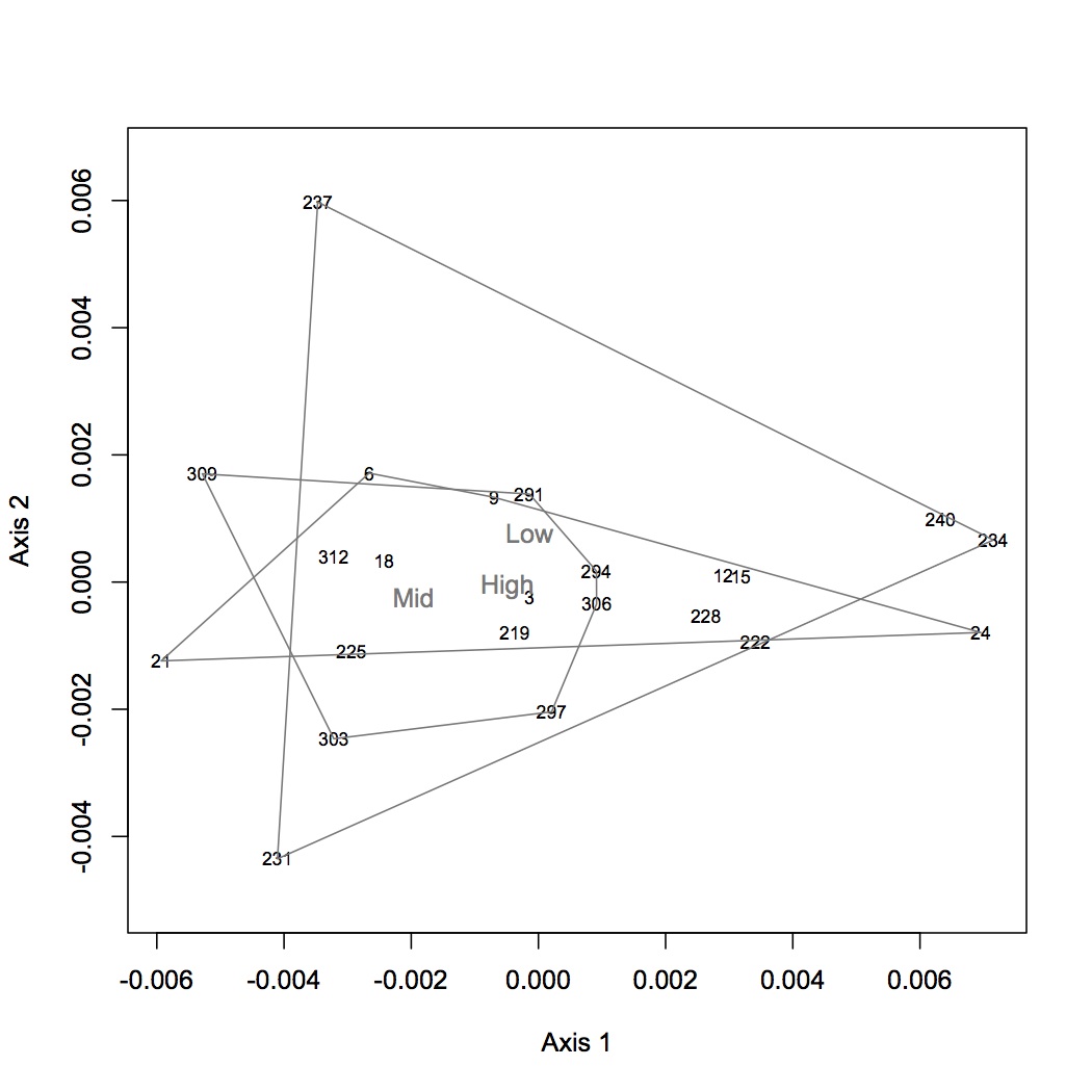
Redid NMDS with new 237 data (sample was diluted and rerun). 237 is no longer an outlier, ANOSIM is still insignificant for among treatment comparison.
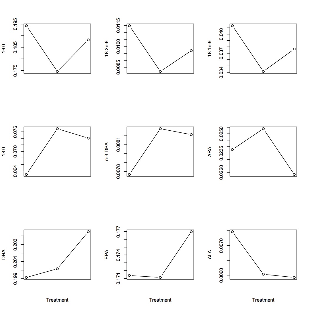
Plotted average FA proportions (each FA is represented as proportion of all FAs) for each of the FAs of interest by treatment. Treatment on the x-axis are in order: Low (400 µatm), Mid (1000), and high (2800). Did ANOVAs for each of these FAs and none were significant.
Secondary Stress:Proteomics
Made a heat map of the proteins that contribute to the high pCO2xMS response. Based on the loadings from the NMDS, determined which proteins were significant in the distribution of oysters in multivariate space for high pCO2 vs. high pCO2xMS. Did the same for low pCO2 and MS so that I could find the overlap of general MS response proteins (those proteins that were significant for MS response at both high and low pCO2). Used skyline peptide data as expression values and made a heat map (non-transformed and log-transformed expression data) for the proteins that were responsible for the oyster response to the combined stressor. The heat map isn't terribly informative so I am not including it here, but the R code is in the proteomics figures for ms script.
February 26, 2013
Bioinformatics: Assignment 7
Downloaded metagenomics fasta file and did blastn (megablast) against ncbi nucleotide database.
./blastn -query /Users/Emma/Documents/module_7/sequences_module7.fa -db /Users/Shared/data/blast/db/nt -out /Users/Emma/Documents/module_7/metagen_blastn -max_target_seqs 1 -outfmt 6 -num_threads 8
In text wrangler, replaced all | with spaces. Uploaded the output file to galaxy and used metagenomics tools to retrieve taxonomic information based on the gene ID in column 3 (e.g. 160338813). On the resulting file, summarized taxonomic data. Most of the sequences are bacteria (9225), followed by Archaea (922), eukaryotes (628), viruses (544), and fungi (155). Drew phylogeny of taxonomic information (saved in evernote).
Ran blastx on metagnomics data.
./blastx -num_threads 8 -out /Users/Emma/Documents/module_7/metagen_blastx -db /Users/Emma/Documents/bioinfo_assignment_1/uniprot_db_010913 -outfmt 6 -evalue 1E-5 -max_target_seqs 1 -query /Users/Emma/Documents/module_7/sequences_module7.fa
Secondary Stress: Shell
Got back the first round of shell data from Gary Dickinson. He did mass and length of both valves as well as nacre area ratio. He is working on hardness tests. For the left valve, the mass was slightly less at 1000 and 2800 µatm compared to 400 (the mean mass was the lowest at 1000), but the differences were not significant. The left valve length was longest at 1000, followed by 2800 and 400, but again not significantly so. The left valve nacre ratio was very similar between 400 and 1000, but lower at 2800 (NS). The mass of the right valve was greatest at 2800 and lowest at 1000 (NS). The right valve length was greatest at 1000 and lowest at 2800 (NS). The nacre area ratio was significantly different among treatments: highest at 1000 and lowest at 400.
February 20, 2013
Secondary Stress: Proteomics
I am trying to determine which proteins are responsible for the different responses to mechanical stress at high and low pCO2. (This work is all saved in the folder "figures for NSA".) To do this, I first joined the lists of peptides (with SPID annotations) that had significant eigen vector loadings on the NMDS (for each pCO2 response to MS) together. I then determined which peptides overlapped between low and high pCO2 and which were unique in the MS response at each treatment. I compared these 2 lists at the protein level and determined which proteins were driving the differing responses at the 2 pCO2. These proteins were then annotated to the GO and GO Slim levels.
February 19, 2013
Bioinformatics: Assignment 6
Joined CDS file for oyster genome to file of methylated CGs to get counts of methylated exons. Will then join this to previous file of methylated CGs, unmethylated CGs, and number of exons, and all CGs all joined to mRNA. I can calculate number of methylated introns from this joining...There are no CGI IDs in the methylated CG file and I would rather work on my NSA talk then learn the necessary steps in Galaxy to fix this problem.
But check out my plots on evernote!
https://www.evernote.com/shard/s242/sh/2843c91e-ebda-45db-a1b6-cdedd65545c3/d0ce0e17d6636eab2590c820fc651af1
https://www.evernote.com/shard/s242/sh/c39fc246-034e-472e-81bc-ea68ada73063/2c5cb70f962826341faa2f23a7f4e14e
February 14, 2013
Bioinformatics: Assignment 6
Using IntersectBed joined bed file of introns to bed file of all CGs and gff file of exons to bed file of all CGs.
./intersectBed -a /Volumes/web/Mollusk/174gm_analysis/Bedtools_Intersect/oyster.v9_90_allCGs -b /Volumes/web/Mollusk/174gm_analysis/oysterv9_90_Introns.bed -c > /Users/emmatimminsschiffman/Documents/Winter_2013/Bioinformatics/CG_Introns
./intersectBed -a /Volumes/web/Mollusk/174gm_analysis/Bedtools_Intersect/oyster.v9_90_allCGs -b /Volumes/web/oyster/bioinformatics/oyster.v9.glean.final.rename.CDS.gff -c > /Users/emmatimminsschiffman/Documents/Winter_2013/Bioinformatics/CG_Exons
I should have been joining files to the mRNA file, not to the all CGs file. I deleted the 4 output files I made today and yesterday and joined methylated CGs, nonmethylated CGs, and exons to the mRNA file. Also joined the mRNA file to the all CGs file. To determine number of CGs, methylated CGs, and nonmethylated CGs, just added the counts in each of the files.
Secondary Stress: Transcriptomics
Enrichment analysis for differentially regulated genes from RPKM data. "Differentially regulated" = 2-fold up or down regulated in high vs. low pCO2 (this was done in excel by dividing the sum of expression at high pCO2 by the sum of expression at low pCO2). These data were then joined with Sigenae annotations from a blastn and SPID annotations of the Signae sequences from a blastx in SQLShare.
SELECT * FROM [emmats@washington.edu].[table_RPKM all oysters.csv]
INNER JOIN [emmats@washington.edu].[table_isotig blastn sigenae v8.txt]
ON [emmats@washington.edu].[table_RPKM all oysters.csv].[Feature ID]=[emmats@washington.edu].[table_isotig blastn sigenae v8.txt].Contig
SELECT * FROM [emmats@washington.edu].[isotig expression with sigenae]
INNER JOIN [emmats@washington.edu].[table_sigenae blastp.txt]
ON [emmats@washington.edu].[isotig expression with sigenae].Accession=[emmats@washington.edu].[table_sigenae blastp.txt].Protein
2 gene lists were used for DAVID: up-regulated at high pCO2 and down-regulated. The background was all the SPID annotations of the contigs. There were no enriched GO Categories in the up-regulated transcripts but there were 70 down-regulated GO categories. REViGO is currently down so cannot make a visualization.
Secondary Stress: Proteomics
Summed the peptide areas from the Skyline output within proteins so that expression values are now by protein and not peptide.
Select Protein, sum(Low1), sum(Low2), sum(Low3), sum(Low4), sum(LowMS1), sum(LowMS2), sum(LowMS3), sum(LowMS4), sum(HighMS1), sum(HighMS2), sum(HighMS3), sum(HighMS4), sum(High1), sum(High2), sum(High3), sum(High4) FROM [emmats@washington.edu].[table_Skyline peptide areas for sql.txt]
Group by Protein
This dataset was then used to do NMDS and ANOSIM and a heatmap in R. The proteome profiles among treatments are significantly different. Annotated the loadings with SPIDS in SQL Share to see if there was enrichment (there was not).
SELECT * FROM [emmats@washington.edu].[table_Workbook2.txt]
INNER JOIN [emmats@washington.edu].[table_Cg proteome db evalue -10.txt]
ON [emmats@washington.edu].[table_Workbook2.txt].ProteinID=[emmats@washington.edu].[table_Cg proteome db evalue -10.txt].Protein
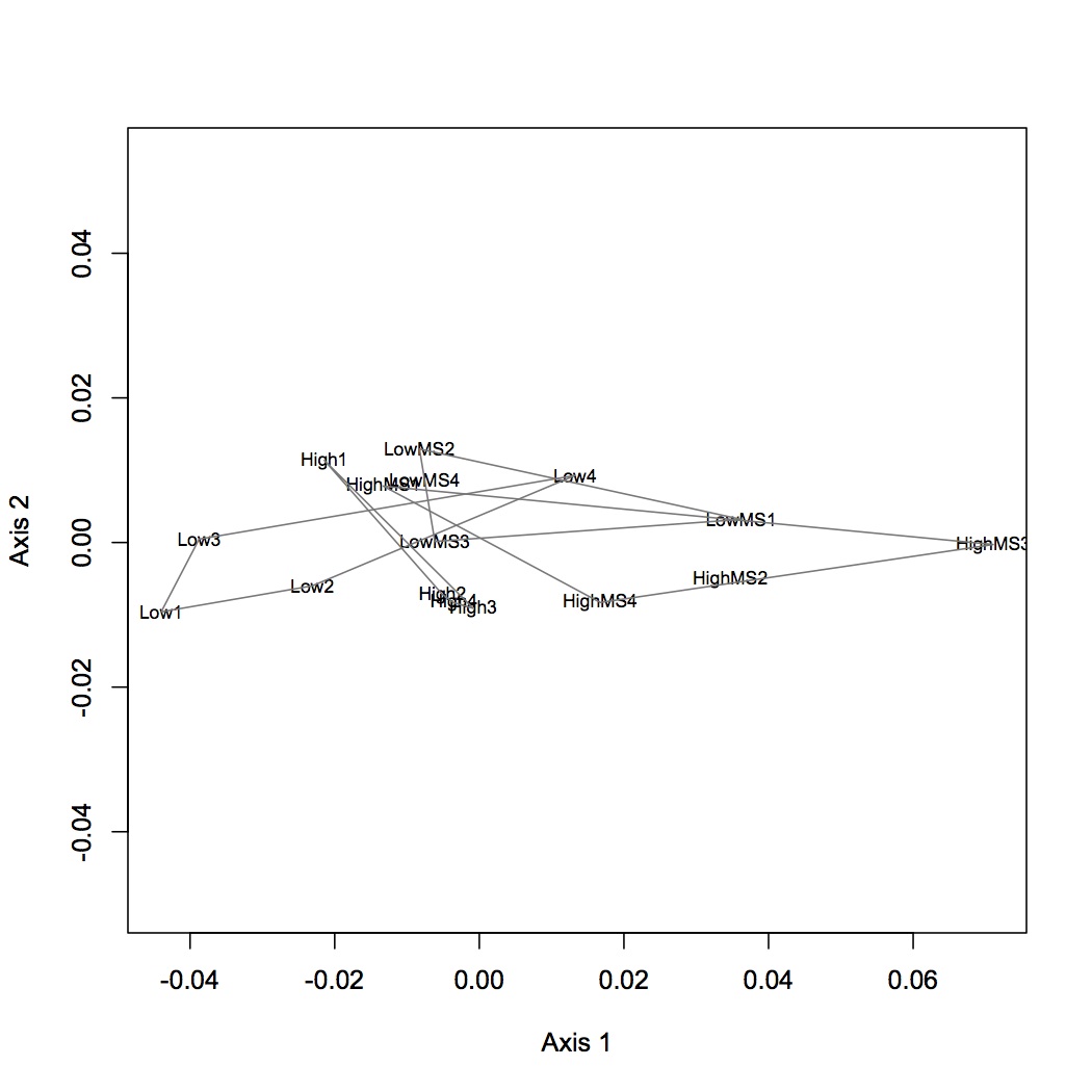
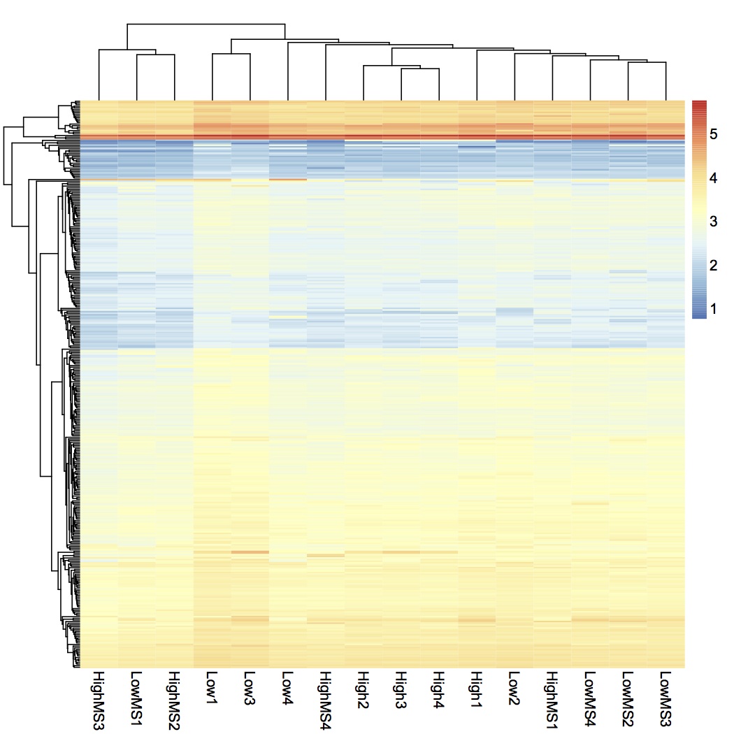
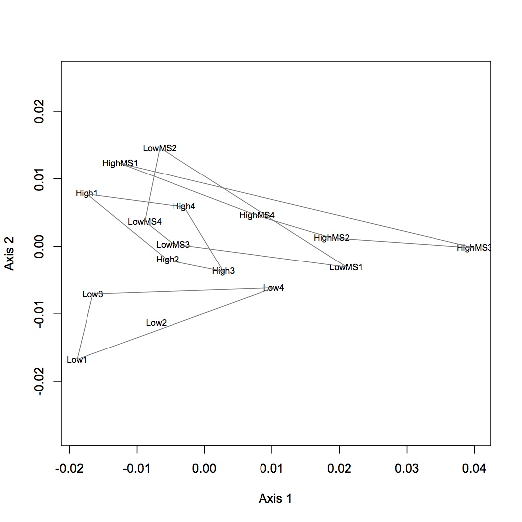
Realized that previous NMDS and ANOSIM of Skyline peptide data was on the untransformed data. Redid NMDS and ANOSIM on log-transformed data. The difference among treatments is still significant.
February 13, 2013
Secondary Stress: Fatty Acids
(this analysis still does not have the new 237 data and oyster 300 was an outlier so is not included)
I redid NMDS and ANOSIM (see 2/6/13) using just fatty acids that are biologically important according to the literature. In the new analysis, the fatty acids included are: 16:0, 18:0, 18:1n-9, 18:2n-6, 18:3n-3, 20:5n-3, 22:4n-6, 22:5n-3, 22:6n-3. There is still no significant difference among the 3 treatment groups. This means that there is more variation due to individual oyster FA profile than due to treatment effect. Interesting note: the appearance of 18:1n-7 indicates bacterial consumption.
Secondary Stress: Proteomics
Took the output from the loading vectors of the Skyline NMDS and joined it with the expression values from Skyline in SQLShare.
SELECT * FROM [emmats@washington.edu].[table_Annotated ProtPep.txt]
INNER JOIN [emmats@washington.edu].[Skyline average peptide areas]
ON [emmats@washington.edu].[table_Annotated ProtPep.txt].[Prot_Pep]=[emmats@washington.edu].[Skyline average peptide areas].[ProtPep]
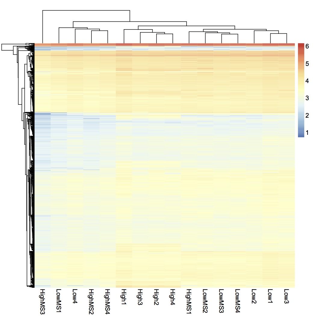
Used just the peptides that had a significant eigen vector loading (p<0.01), log transformed those data, and made a heat map using pheatmap in R.
Bioinformatics: Assignment 6
Downloaded bedtools and Xcode 4.6. Navigated to bedtools file using Terminal and ran "make". Ran intersectbed on file of all CGs in genome and all methylated CGs in oyster genome. This will show which CGs in entire genome are methylated. I did the same thing except with unmethylated CGs in entire genome and all CGs.
./intersectBed -a /Volumes/web/Mollusk/174gm_analysis/Bedtools_Intersect/oyster.v9_90_allCGs -b /Volumes/web/Mollusk/174gm_analysis/MethylatedCG_BED.bed -c > /Users/emmatimminsschiffman/Documents/Winter_2013/Bioinformatics/All_CGs_MethylatedCG
./intersectBed -a /Volumes/web/Mollusk/174gm_analysis/Bedtools_Intersect/oyster.v9_90_allCGs -b /Volumes/web/Mollusk/174gm_analysis/NoMethCG_BED.bed -c > /Users/emmatimminsschiffman/Documents/Winter_2013/Bioinformatics/All_CGs_NonMethCG
February 12, 2013
Secondary Stress: Fatty Acids
Retrieved freeze dried samples and GC-ready samples from CEE. They are now in the -20°C behind Sam's bench. Sean ran the 50% diluted 237 today and is sending me the data.
Olympia Oyster Epigenetics
Added 175µl water to digestion-ligation that went overnight. Used this template to do a pre-select PCR (the protocol has been modified to use AmpliTaq). For each reaction: 4 µl digested DNA, 2.5 µl 10X AmpliTaq buffer (no MgCl2 added), 2 µl 10 mM dNTP, 0.2 µl AmpliTaq, 1.75 µl 50 mM MgCl2, 0.6 µl 10 µM preselect EcoRI primer, 0.6 µl 10 µM preselect H/M primer, 12.35 µl H2O (20 µl master mix and 4 µl template per well). Cycling parameters: 72 °C 2 minutes; 25 times 94°C 30s, 56°C 30s, 72°C 2 minutes; 60°C 30 minutes (saved as PRESEL on 96-well plate thermalcycler).
Made 1% agarose gel with EtBr. Mixed 10 µl of PCR product with 3 µl of Bioline 5x loading dye. Ran negative control for Msp and CAS.001 and DAB.087 for both Msp and Hpa. Gel ran for ~30 minutes at 100 V. Gel photo: https://www.evernote.com/shard/s242/sh/3672bf89-2caf-4501-aa46-9ad619826ca0/fc3a1962cbb52144fd1e4abc32bf292a
There were smears in all 4 samples and nothing present in the negative control.
Proceeded to select PCR. I am only PCRing a subset of samples to test out the select primer pairs. Mac previously ordered 7 primer pairs so I am making sure that they work well with Olys. Primer pairs are listed in the table below and each primer is designated by a specific 3-nucleotide tag. H/M TCG and TGC may be mixed up. Select PCR was done using the same recipe as preselect PCR and the same cycling parameters. PCR plate layout can be found here: https://www.evernote.com/shard/s242/sh/2fe19c66-17f9-4757-872d-1ea789cd9430/c13eb04c4d23084f67658ab932f4f7e6
| Pair |
EcoRI primer |
H/M primer |
| 1 |
AAC |
TTA |
| 2 |
ACA |
TTC |
| 3 |
ACA |
TGA |
| 4 |
ACA |
TGT |
| 5 |
ACA |
TGC |
| 6 |
ACA |
TAC |
| 7 |
ACG |
TCG |
Ran the samples on a 1.5% agarose gel with EtBr at 100V for ~40 minutes. All primer pairs amplified the pre-select PCR product. I tested both DAB.091 samples and both of them had amplification. Gel image here: https://www.evernote.com/shard/s242/sh/6738a26d-4fe1-43f7-a026-2baa830cb1a5/2d45335c74a81f02ce632f4847df4183
February 11, 2013
Olympia Oyster Epigenetics
Finished 3 DNA extractions started yesterday. See 2/8/13 for details. There is still not pellet in DAB.091, but continued with extraction anyway. The 2 FID samples were resolubilized in 200 ul of water and DAB.091 with 100 ul. Nanodrop data
DAB.091 still has a very low concentration, but the other 2 samples are much better. Going forward I will probably analyze both extracted samples of DAB.091 and just the new FID.97 and FID.100.
Day 2 of MSAFLP protocol. Made dilutions of adapters in T4 ligase buffer:
Hpa/Msp adapters = 4.2 µl H/M adapter I, 4.2 µl H/M adapter II (both at 0.24 ng/µl), 5 µl 10x T4 ligase buffer, 36.6 µl H2O.
Eco RI = 3.7 µl Eco adapters I and II (at 0.27 ng/µl), 5 µl 10x T4 ligase buffer, 37.6 µl H2O.
Incubated adapter mixes at 95°C for 2 minutes and let cool for 45 minutes on benchtop. Realized at next step that I did not have enough of the H/M adapter, so I made 2x more batches of it as described above.
Made dilutions of T4 ligase and Eco RI adapter:
T4 ligase = 1 uL T4 ligase, 50 ul 10x T4 buffer, 449 ul H2O.
EcoRI adapter = 10 ul EcoRI (40 pm/ul, see above), 90 ul H2O
Digestion-ligation reactions were prepared in a PCR plate and details can be found in the digest-ligation tab of this spreadsheet. Samples in bold had low DNA concentrations so the max volume possible (15 µl) was used for the reactions. NaCl was prepared from Mac's stock of 2000 mM (125 µl of Mac's Stock + 75 µl water). Samples are laid out in order on the PCR plate, starting with CAS.001 in A1 and a negative control in the last spot (H4) for MspI. HpaII digestions have the exact same layout except can be found in columns 5-8 on the plate.
February 10, 2013
Olympia Oyster Epigenetics
Began digestion of 3 samples that did not yield enough DNA on Friday: FID.097, FID.100, DAB.091 (see 2/7/13 for details).
February 8, 2013
Secondary Stress: Fatty Acids
This morning I picked up the data that Sean re-ran for me (samples 9 and 300). I also diluted sample 237 1:1 in hexanes to be re-run. Sample 300 looks like it might still be unusable, but I need to look at it more closely.
Secondary Stress: Proteomics
Continuation of analysis of Skyline data. Exported the eigen vector loadings from R for the NMDS done yesterday. Annotated the proteins with SPIDs in SQLshare.
SELECT * FROM [emmats@washington.edu].[table_loadings from skyline nmds.txt]
INNER JOIN [emmats@washington.edu].[table_Cg proteome db evalue -10.txt]
ON [emmats@washington.edu].[table_loadings from skyline nmds.txt].Protein=[emmats@washington.edu].[table_Cg proteome db evalue -10.txt].Protein
The SPIDs will be used in DAVID to look at the enrichment of GO terms and KEGG pathways for the proteins associated with peptides that have significant loadings (p< or = 0.01) compared to all the peptides used in the Skyline analysis. There were no enriched GO terms or pathways in this protein set.
Olympia Oyster Epigenetics
Finished extractions of DNA started yesterday. Spun samples at 10,000xg for 10 minutes and removed supernatant to a new tube. Added 0.5 mL 100% EtOH and inverted tubes 8 times. Stored for a few minutes at RT. Sedimented DNA by spinning for 5 min at 5,000xg. Washed DNA pellets 2x with 1 mL of 75% EtOH, inverting a couple of times to really wash pellet. Dissolved pellets in 200 µl Nanopure H2O. Could not see pellets in samples FID.100 and DAB.091, I think I lost the pellet in FID.097. All of these samples have low concentrations so I will extract them again.
Nanodrop data is below. Samples were stored at -20C in box started May 2011.
Nanodrop
February 7, 2013
Secondary Stress: Proteomics
Finished visualization of analysis done 2/5/13 - comparison of enriched processes in response to MS at 2 different pCO2 levels. Pie charts show the number of proteins that contribute to each enriched GO Slim category. There is very little difference between the 2 treatments.
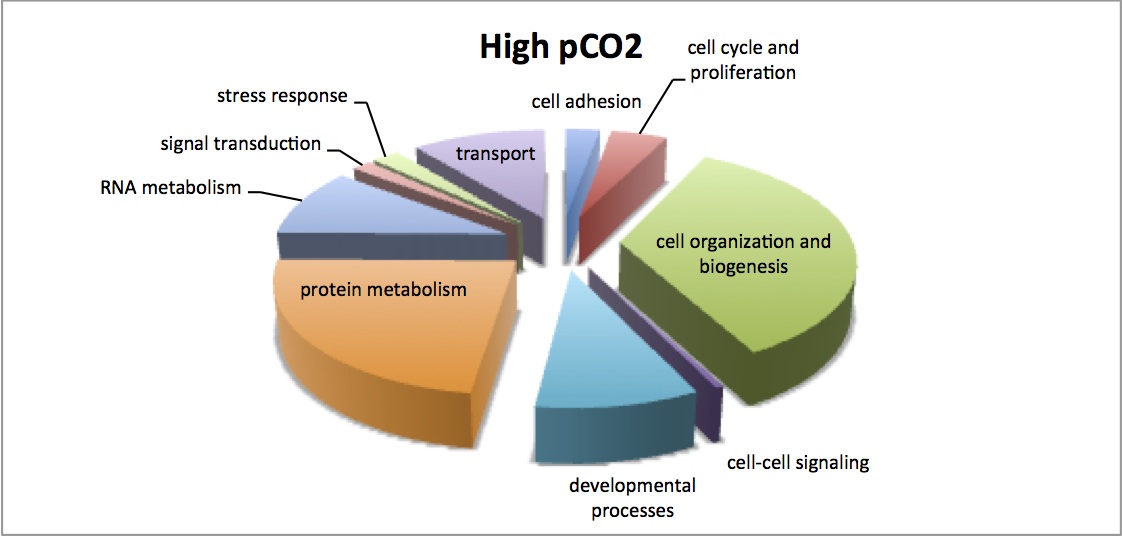
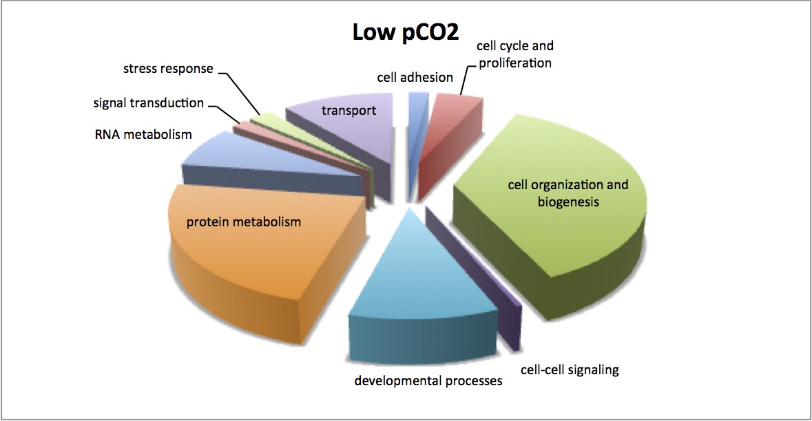
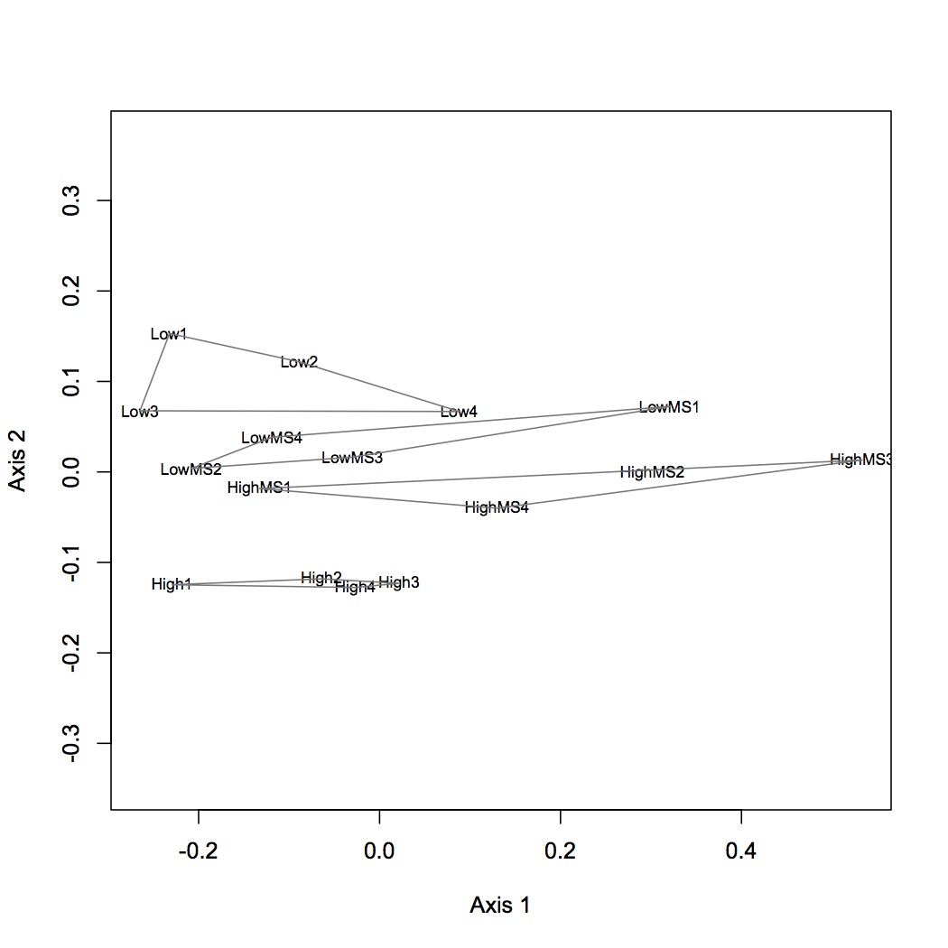
NMDS of all proteomic samples shows that there are differences in the proteomic profiles of the LowMS and HighMS oysters, which may mean that responses to MS are different at the different pCO2. Dropped low abundance proteins and did log(x+1) transformation, bray-curtis dissimilarity coefficient. ANOSIM showed no significant difference between these 2 groups (R=0.05208, p=0.355). I redid the analysis without dropping low abundance proteins and got the same result.
Analysis of Skyline data - in Excel calculated average areas for peptides for each oyster. This was accomplished by creating pivot tables (1 for each oyster) with the protein-peptide name as the descriptor and the average total area (across technical replicates) as the value. Joined all of these tables together in SQLshare.
SELECT * FROM [emmats@washington.edu].[table_average areas for lowpCO2 and MS.csv]
INNER JOIN [emmats@washington.edu].[table_average areas for highpCO2MS.csv]
ON [emmats@washington.edu].[table_average areas for lowpCO2 and MS.csv].ProtPep=[emmats@washington.edu].[table_average areas for highpCO2MS.csv].ProtPep
SELECT * FROM [emmats@washington.edu].[skyline joining 1]
INNER JOIN [emmats@washington.edu].[table_average areas for highpCO2.csv]
ON [emmats@washington.edu].[skyline joining 1].ProtPep=[emmats@washington.edu].[table_average areas for highpCO2.csv].ProtPep
Used this joined file to do a NMDS and ANOSIM. Data were Log(x+1) transformed and the bray-curtis dissimilarly coefficient was used. There is a significant difference among the treatment groups (p=0.001).
Olympia Oyster Epigenetics
Began DNA extractions of oyster mantle tissue that Katie collected previously (n=10 oysters each from Case Inlet, Dabob Bay, and Fidalgo Bay). All tissues were subsampled except for DAB_90, DAB_95, and CAS_004, which were used in their entirety. 0.5 mL of DNazol was added to <100 mg of mantle tissue and homogenized with a sterile pestle. Then 0.5 mL more DNazol was added along with 2.35 µl proteinase K and tubes were mixed by manually shaking them. Extractions were incubated overnight on the shaker at room temperature.
February 6, 2013
Secondary Stress: Fatty Acids
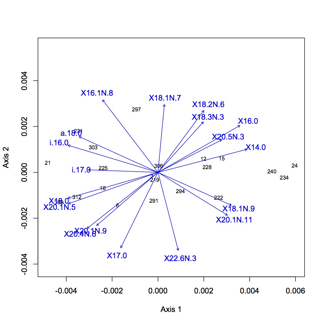
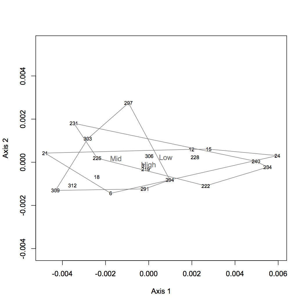
I identified the peaks in all the chromatograms. Sample 237 chromatogram looks odd (missing a lot of peaks, really hard to score peaks that are there) - it may need to be diluted (when included in the NMDS it is obviously a far outlier). I will run it again next week. The current dataset does not contain samples 237, 300, or 9. (Sean re-ran 300 and 9 last night.) For each oyster, I divided each peak area by the total peak areas for all identified fatty acids. This gives the relative proportion of each fatty acid. This dataset was log(x+1) transformed and NMDS was performed using a Bray-Curtis dissimilarity coefficient. ANOSIM was also performed to assess significance of treatment on FA profile. There was no significant difference among groups. The first NMDS shows loading that are significant at the p<0.01 level. The next step will be to focus on specific FAs of interest (based on the literature) and do ANOVAs.
February 5, 2013
Secondary Stress: proteomics
From Enrichment analysis done yesterday, uploaded the list of enriched GO terms and joined to GO Slim terms in SQLshare.
SELECT * FROM [emmats@washington.edu].[table_NMDS no low abundance proteins enriched loadings.csv]
INNER JOIN [sr320@washington.edu].[GO_to_GOslim]
ON [emmats@washington.edu].[table_NMDS no low abundance proteins enriched loadings.csv].[GO Number]=[sr320@washington.edu].[GO_to_GOslim].[GO_id]
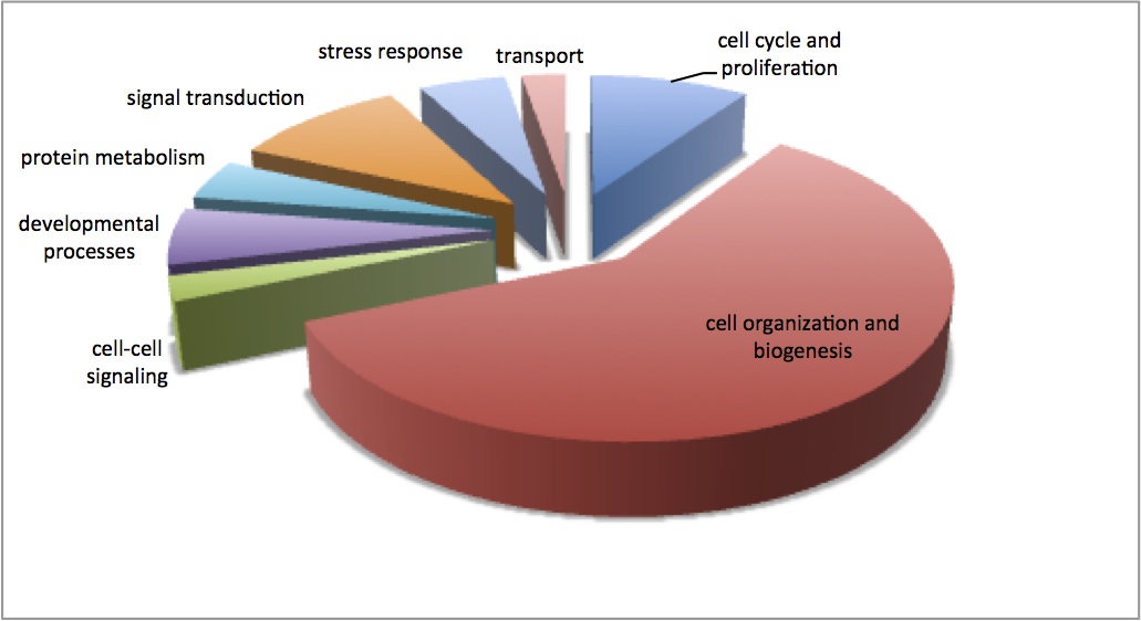
Below is the pie chart showing the enriched GO Slim categories for this dataset. The pie was constructed from the number of contigs that contributed to each enriched GO Slim term.
Did the same enrichment analysis as described yesterday - enrichment of significant loadings for the proteomic NMDS that does not include low abundance proteins. This time, I selected the Kegg Pathway output to look at the pathways that are overrepresented in this dataset. 10 pathways were enriched: glycolysis/gluconeogenesis, glyoxylate and dicarboxylate metabolism, fructose and mannose metabolism, ribosome, citrate cycle (TCA cycle), proteasome, cardiac muscle contraction, galactose metabolism, butanoate metabolism, oxidative phosphorylation.
Using NMDS and loadings of proteins on the NMDS axes, I am doing a comparison of the effects of pCO2 on response to mechanical stress (MS). I did NMDS for isolated pCO2 groups, i.e. highpCO2 and highpCO2 + MS. I created files of the eigenvector loadings and joined these to SPID annotations of the C. gigas proteome in SQLshare (example code below).
SELECT * FROM [emmats@washington.edu].[table_eigen loadings lowpCO2 MS.txt]
INNER JOIN [emmats@washington.edu].[table_Cg proteome db evalue -10.txt]
ON [emmats@washington.edu].[table_eigen loadings lowpCO2 MS.txt].Protein=[emmats@washington.edu].[table_Cg proteome db evalue -10.txt].Protein
Joined the GO terms with GO Slim terms to compare enrichment between pCO2 treatments.
Secondary Stress: Fatty Acids
Sean helped me identify peaks in my results so that I know which fatty acids I'm looking at. I also got all of my raw data off the computer in CEE and onto Eagle. I need to go through all 24 samples and identify the peaks so that I can compare relative amounts of specific fatty acids among treatments. 2 of the samples need to be re-run: 300 and 9. 300 had a lot of extra peaks, possibly due to being too concentrated. I diluted it 1:1 in hexanes to rerun. 9 was run right after 300 and looks fine except one peak is much fatter than it should be and so cannot be reliably quantified. This could be an artefact of being run after a concentrated sample or it could be because 9 was the sample that I added too much H2SO4 to and had to modify its extraction.
February 4, 2013
Bioinformatics: Assignment 4
The blastx I ran on Friday (2/1) finished without any errors but the output file does not seem to exist anywhere so I am using SR's blastx results for the transcriptome backbone. In SQLshare, I joined the blastx results with the DESeq results from 2/1/13. I used the entire list of SPIDs that matched to contigs as the backbone for DAVID (v 6.7) and the SPIDs that corresponded to differentially expressed contigs as my gene set (adjusted p-value less than or equal to 1E-5). Redundant SPIDs were removed from both lists. I uploaded these lists to DAVID and downloaded the chart for Gene Ontology GOTERM_BP_FAT. I entered the GO numbers and associated p-values in revigo to visualize the enriched GO biological processes in the differentially expressed genes (n=56). Many of the enriched processes are involved in reproduction, which makes sense since I compared male and female samples. REvigo visualization is here: https://www.evernote.com/shard/s242/sh/093ec8c2-fcd3-41b3-afdb-5941778fdcee/fe313ad44eeb1328863cac0a9880546c
Secondary Stress: Proteomics
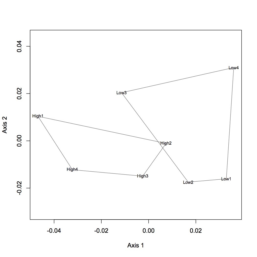
Did a NMDS and ANOSIM on the oysters that were exposed to just pCO2 stress (no MS). Used the protein-level data. There is no significant difference between treatments, but there is a shift in expression in the proteome in response to pCO2.
Used loadings file from 2/1/13 and joined with Cg proteome blastx results in SQL share.
SELECT * FROM [emmats@washington.edu].[table_no low abundance sig loadings.csv]
INNER JOIN [emmats@washington.edu].[table_Cg proteome db evalue -10.txt]
ON [emmats@washington.edu].[table_no low abundance sig loadings.csv].protein=[emmats@washington.edu].[table_Cg proteome db evalue -10.txt].Protein
The background for DAVID is the SPIDs from the file Cg proteome db evalue -10 (so low abundance proteins are not excluded) and the "gene" set is taken from the significant loadings mentioned above. 52 gene ontology terms were enriched (GOTERM BP FAT). VIsualization in revigo can be seen in evernote: https://www.evernote.com/shard/s242/sh/a25e7b20-6531-483d-bcc3-04c3d64e13e9/77de8e809f0a1f71f5f6c1eaad50b1ae. Downloaded R code to make better plot.
February 3, 2013
Secondary Stress: Fatty Acids
Removed last 8 samples and replaced caps before storage at -20°C. Turned off air and H2 gas cylinders.
February 2, 2013
Secondary Stress: Fatty Acids
Removed the samples run yesterday and replaced caps (caps used in run have a hole in them from the autosampler which could lead to evaporation during storage). Loaded last 8 samples to run.
February 1, 2013
Secondary Stress: Fatty Acids
The samples did not run yesterday because the hydrogen was not turned on for the GC. I turned on the H2 this morning and restarted the samples.
Secondary Stress: Proteomics
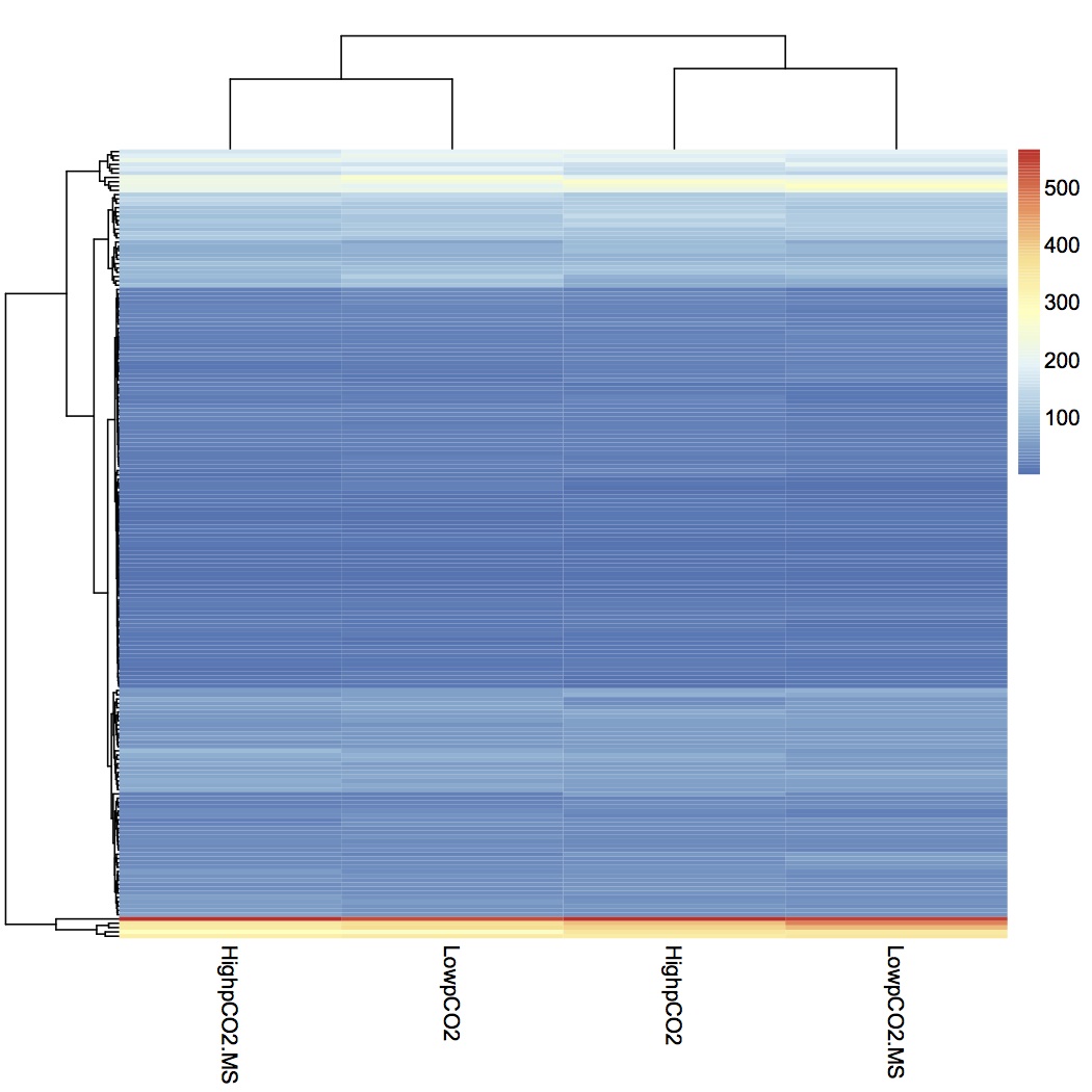
Took list of proteins that had significant NMDS loadings (in folder "for heat map") where significant means p < or = 0.01 and joined with spectral counts in SQLshare. From this file, created an input file to make a heat map using pheatmap in R. clustered both rows and columns using average linkage and euclidean distance. There is no obvious pattern in the expression of these proteins within treatment groups.
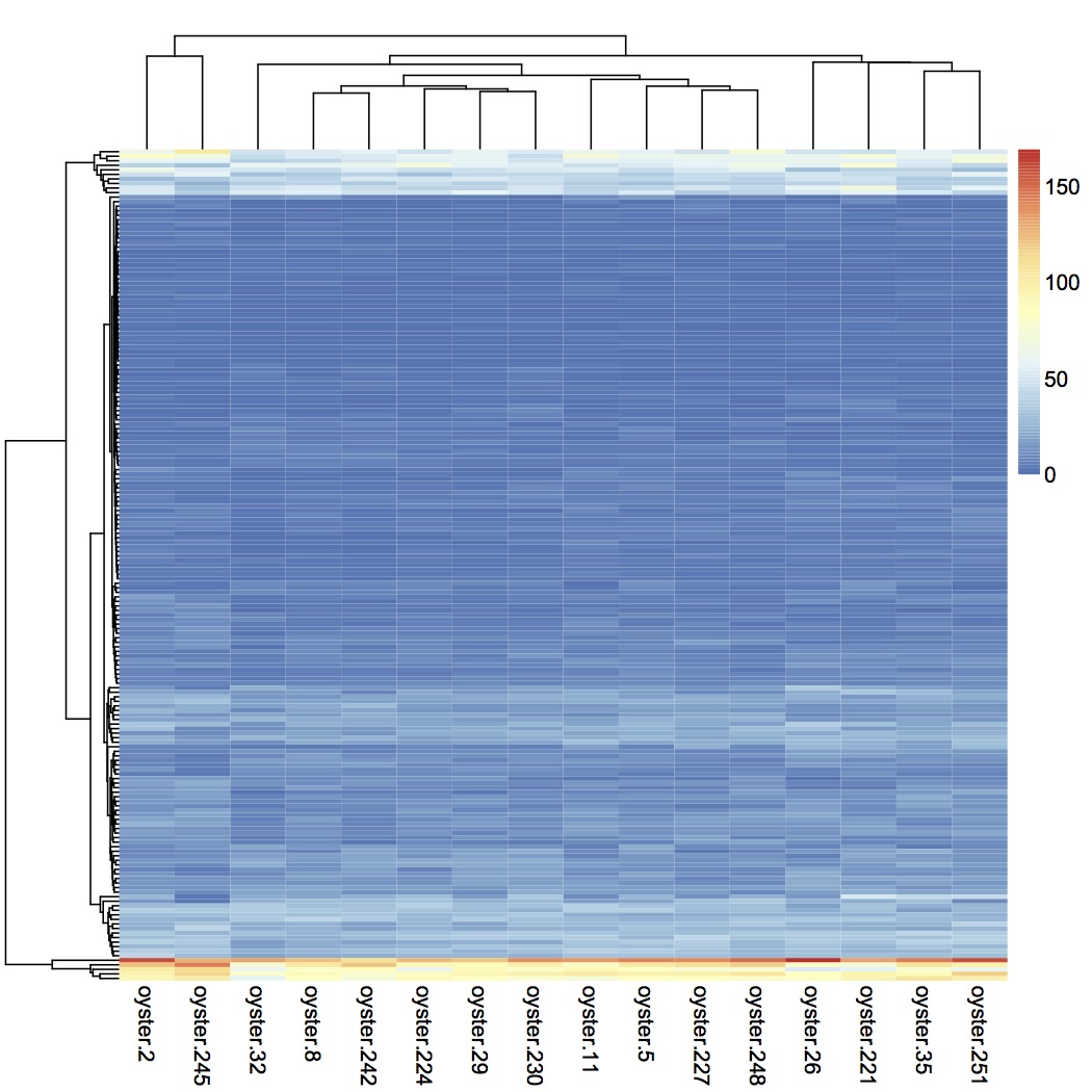
Summed spec counts within the 4 treatment groups and made a heat map from that input file.
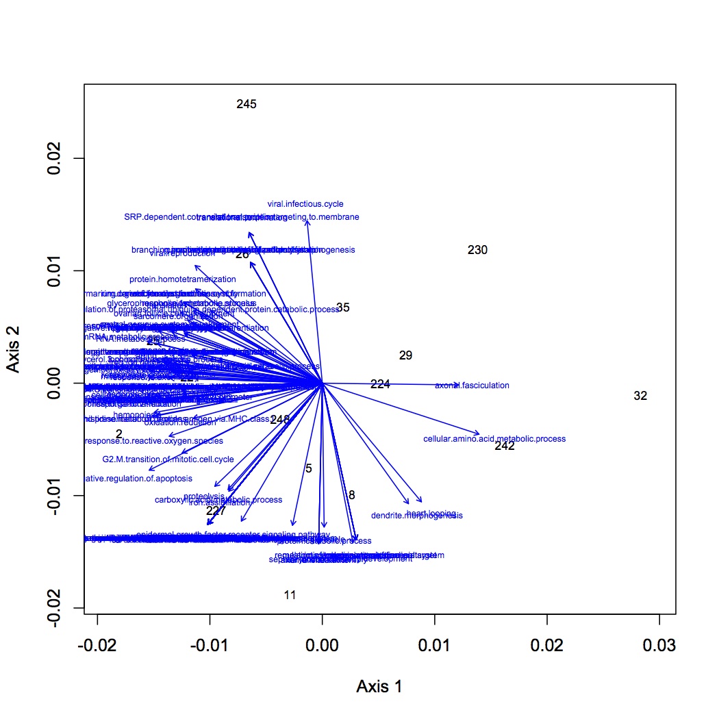
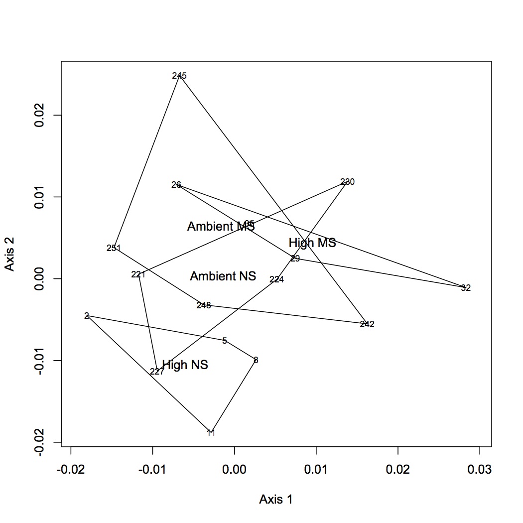
Did NMDS for proteomics at GO Slim level. There was no significant effect of treatment on proteome expression.
Bioinformatics: Assignment 4
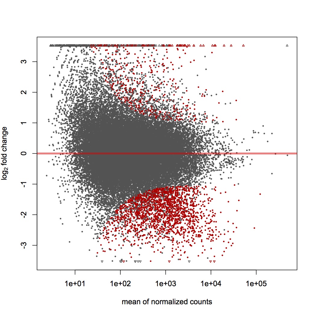
Took Steven's mapped reads (http://eagle.fish.washington.edu/cnidarian/fish546/fish546_CLCexperiment_readcounts.xls) and created a file of total reads for each sample (male 106, male 108, female 106, female 108). Only kept contigs that had at least 10 reads across all 4 samples. Did DESeq on dataset (genes in red are differentially expressed).
Began blastx of backbone used in SR's assembly against the SwissProt database made 1/9/13. E-value cutoff = 1E-5, only return the top hit.
./blastx -num_threads 8 -out /Users/Emma/Documents/module_4/blastx_output -db /Users/Emma/Documents/bioinfo_assignment_1/uniprot_db_010913 -outfmt 6 -evalue 1E-5 -max_target_seqs 1 -query /Users/Emma/Documents/module_4/backbone.fa
January 31, 2013
Secondary Stress: Fatty Acids
Results from GC-FID run yesterday look good. All FA peak sizes are <100 (as measured on the y-axis), which indicates that the samples do not have to be diluted. Printed results.
Began GC-FID of next 8 samples.
January 30, 2013
Secondary Stress: Fatty Acids
Finished transmethylation of samples run yesterday. Chose 8 samples (3 each from first 2 extraction days and 2 from today) to run overnight on the GC-FID. The program used to run the samples is called FAMES4.
Secondary Stress: Proteomics
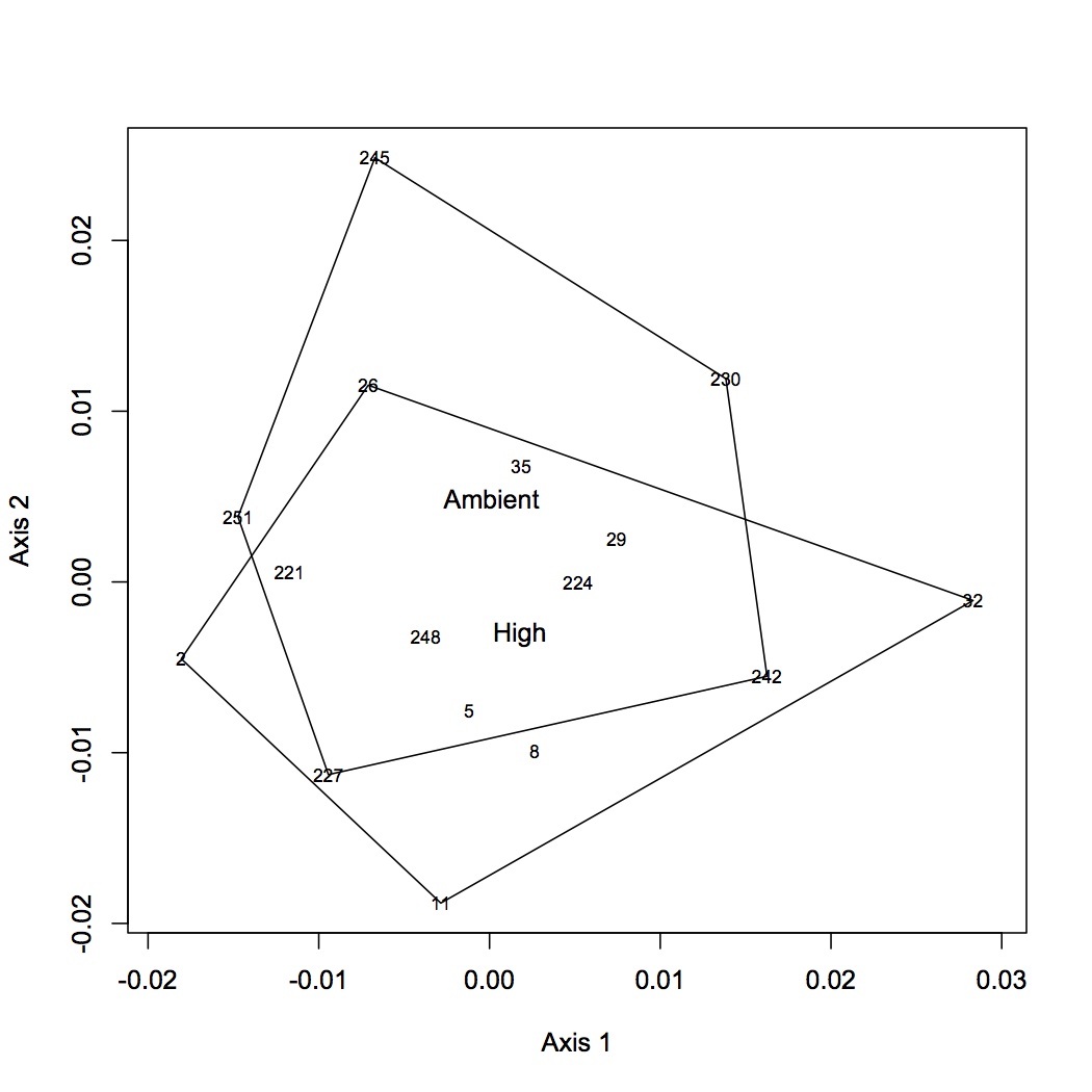
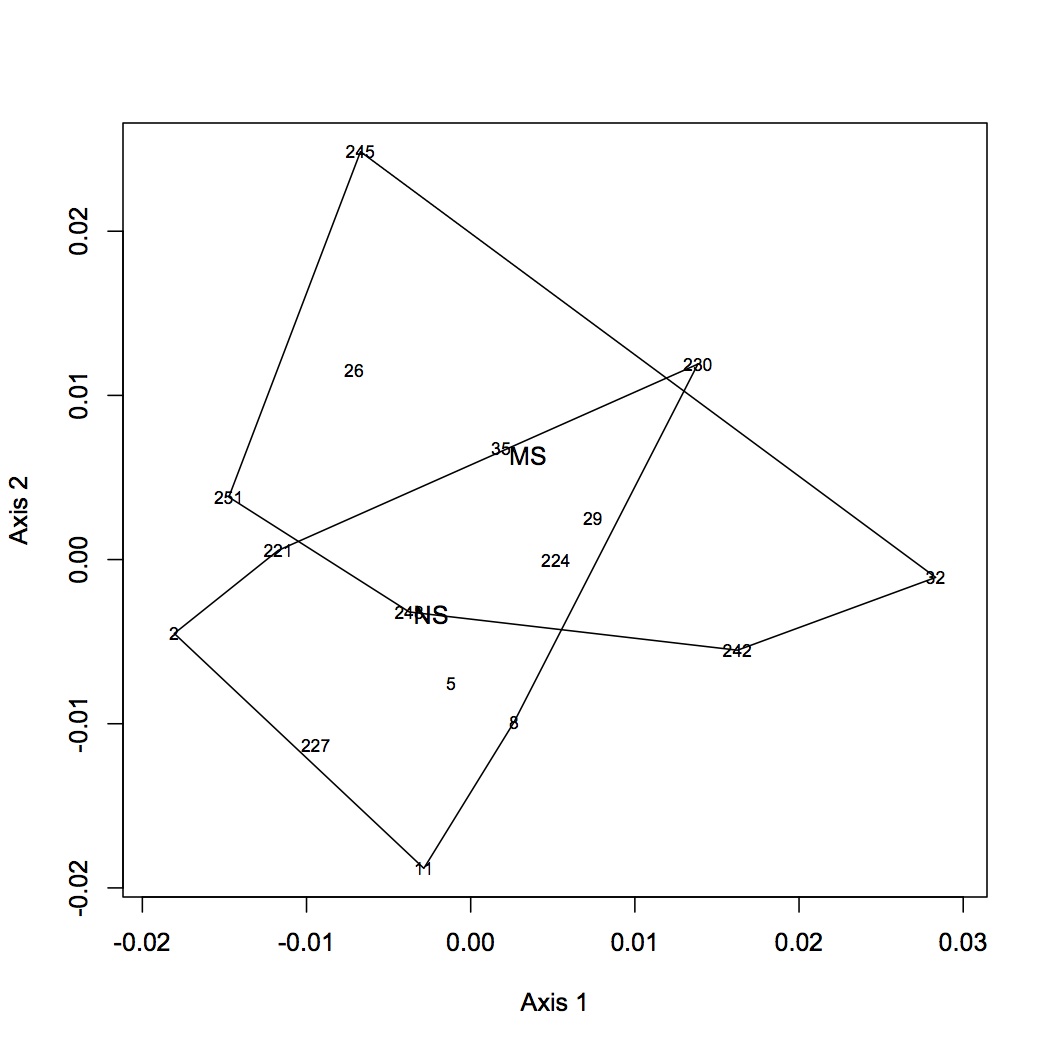
Created a file of the summed spectral counts for GO terms. Only those proteins that had a blastx result of less than or equal to 1E-5 were included. Made sure to get rid of redundancy in protein-GO term pairings. Based on ANOSIM, there is no difference in the proteome from pCO2, MS, or a combination of the 2. This is different from the same analysis done earlier with an older version of GO associations.
January 29, 2013
Secondary Stress: Fatty Acids
Began extractions of the last 8 oysters: Exp2.6, 15, 18, 219, 222, 225, 291, 309. Samples were left in 50°C water bath overnight and transmethylation will be finished tomorrow.
January 28, 2013
Secondary Stress: Proteomics and RNA-Seq
Joined tables in SQLshare to annotate proteome and transcriptome to GO Slim level. Queries for the joining can be found in my evernote (https://www.evernote.com/Home.action#st=p&n=66b4781b-152a-4a13-b275-6688b3fd3ede).
January 24, 2013
Bioinformatics: Assignment 3
Hummingbird had to be rebooted, so I re-ran the code from yesterday with one change: decreased the jellyfish memory from 20,000 G to 2,000 G.
Hummingbird does not have enough disk space to run Trinity
I downloaded the data file and trinity to the mac mini. I entered the exact same code as I did on Hummingbird (using 2,000 G for jellyfish memory) and I got the error below.
Can't exec "/Users/Emma/Desktop/trinityrnaseq_r2012-10-05/trinity-plugins/jellyfish/bin/jellyfish": No such file or directory at ./Trinity.pl line 1311.
Error, cmd: /Users/Emma/Desktop/trinityrnaseq_r2012-10-05/trinity-plugins/jellyfish/bin/jellyfish count -t 2 -m 25 -s 306783378285 --both-strands single.fa died with ret -1 at ./Trinity.pl line 1315.
I forgot to run "make" to set up the trinity app. After doing that, Steven got the code to work and it is running.
With Claire, I started an assembly of the same data on CLC. We tried trimming it first, but trimming just got rid of >99% of the data, so we are assembling the untrimmed reads with a minimum contig length of 200 (see her notebook for more details).
January 23, 2013
Secondary Stress: Fatty Acid
Started next group of fatty acid extractions, samples = Exp2.9, 24, 228, 231, 234, 294, 300, 306. Took samples all the way through incubation at 50°C overnight (in transmethylation procedure). Samples sat for ~1 hour before being sonicated the first time because someone else was using the sonicator. For the 2 mL addition of 1% H2SO4 in MeOH (transmethylation procedure), the pipette lost its vacuum and 10 mL fell into sample 9. Tomorrow I will divide this sample into 3 separate tubes and continue the extraction on all 3, combining the separate fractions at the end.
Secondary Stress: Proteomics
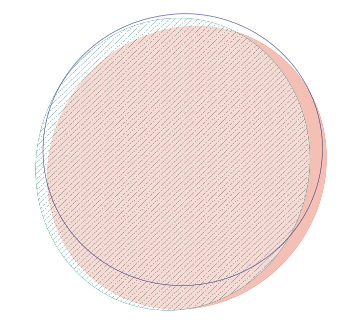
Made venn diagrams to compare biological variation within treatments. Used 3 of the 4 oysters for each treatment and figured out in how many oysters each protein was identified. Used EulerAPE to make the venns. Only the venn diagrams for high pCO2 + MS and low pCO2 + MS were exact. The venn diagrams pretty much looked the same across treatments. The one for high pCO2 + MS is below. Proteins used had at least 10 spectral counts across all oysters.
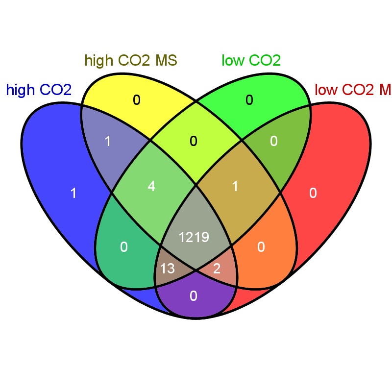
Used Venny to create a diagram comparing the proteins identified across all 4 treatments. Proteins used for the Venn had at least 10 spec counts across all oysters.
Uploaded files to SQL Share, which will take the place of Galaxy. Files uploaded are to redo GO-based analyses for proteomics and transcriptomics for the manuscript.
Bioinformatics: Assignment 3
For this module (assembling HTS data) I'm going to learn Trinity. I downloaded the smaller of the 2 sample datasets (SE_sm_filtered...) onto Hummingbird and put it in my documents folder. This file is single-end Illumina HiSeq.
Command line for Trinity out of trinityranseq_r2012-10-05 directory: fastq file, use 20000G of memory, single end data, min contig length of 200
./Trinity.pl --seqType fq --JM 20000G --single /Users/Emma/Documents/module_3/SE_sm_filtered.fastq --output /Users/Emma/Documents/module_3/Trinityout_012313 --min_contig_length 200
January 22, 2013
Secondary Stress: Fatty Acid
Finished extraction of samples started yesterday (transmethylation). Stored autosampler vials at -20°C.
Secondary Stress: Proteomics
Finished file preparation for venn diagrams (see 1/21/13).
Uploaded Mouse Genome GO Slim file to Galaxy (http://www.informatics.jax.org/gotools/data/input/map2MGIslim.txt).
Created a file of all spec counts (summed across tech reps for each oyster, at least 10 spec counts for each protein) to join with new GO annotations. SPID annotations are from previous blastx (file = Cg proteome db evalue -10). Joined with SPIDs, new GO file (1/18/13) and new GO Slim file.
January 21, 2013
Secondary Stress: Fatty acid
First round of fatty acid extractions on freeze-dried samples (1/15/13): Exp2.3, 12, 21, 237, 240, 303, 312, 297. Followed protocol uploaded 1/10/13. Before weighing out 2.5 mg of freeze dried tissue, mixed the samples around to try to get a representative sample of all that was homogenized. Sample 21 broke in the centrifuge after the first fraction had been removed (i.e. after addition of 2.7 mL chloroform). Continued with extraction of just the 1 fraction of 21 but may re-extract it later since the second fraction does contain a good concentration of FAs, although the first has the large majority. Left samples in 50°C water bath overnight.
Secondary Stress: Proteomics
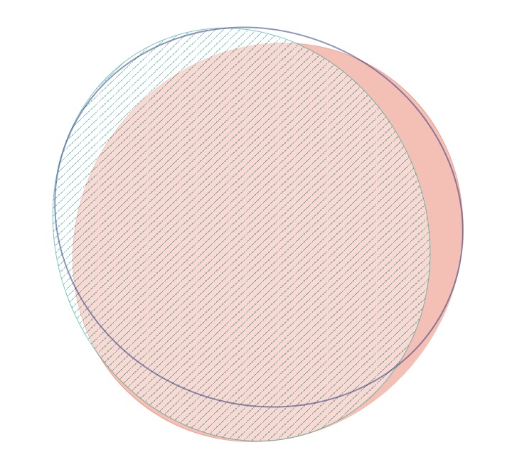
I am making Venn diagrams to show the overlap in proteins identified across technical replicates. For each oyster (3 technical replicates), I created a backbone of non-redundant protein IDs that were sequenced across all replicates. I then joined each replicate file to the backbone and kept only proteins that had at least 3 spectral counts across the 3 tech reps. I found the number of proteins that were identified in all 3 replicates, those that were in just 2 replicates, and those found in a single replicate. So far I have only done this for oysters 101B2, 5, 8, and 11 because Galaxy has stopped working. I used eulerAPE to make the venn diagrams. For all 4 oysters so far, the venns were inexact. An example (for 101B11) is below. While making the input files for the venn diagrams, I found that files 101B11_01 and 101B11_03 had not been edited correctly and so previous analyses using these files might be incorrect (the protein ID column still had multiple proteins per cell, separated by commas).
January 18, 2013
Secondary Stress: Proteomics and RNA-Seq
Continuation of acquiring and editing new GOA files. Uploaded both information and association files from EMBL into Galaxy (selected "tabular" as file format, this is necessary to make Galaxy recognize columns). for the gp_information file, cut the first 18 lines of the file. Then removed columns 1, 2, 7,8,9,10, and 11. Named this file swissprot gene information 011813. Removed the first 19 lines (header) of the gp_association file and edited the file so that only the columns containing the SPID and GO term remained (swissprot goa 011813).
Bioinformatics: Assignment 2
Joined blastx file with new swissprot info and GOA files (see above). Exported and created file of just the GO terms - uploaded this file to cateGOrizer.
MeDip
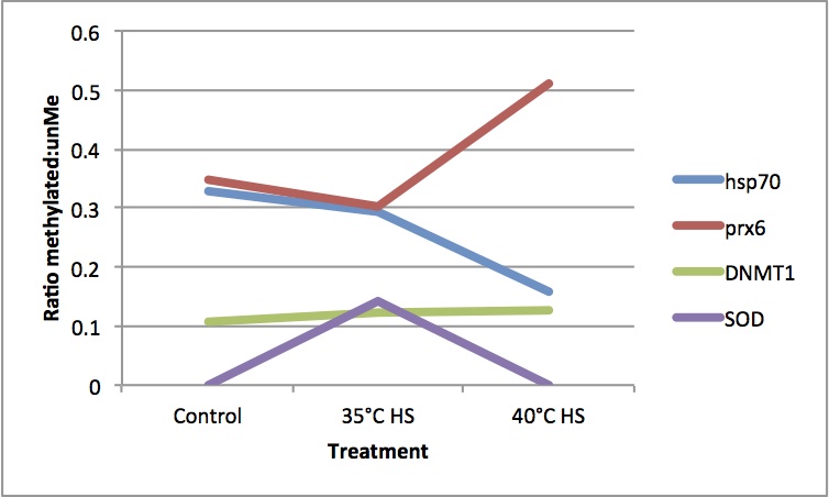
Here are the results from yesterday's medip. It looks like methylation status varies for the genes at the different temperature treatments.
January 17, 2013
Bioinformatics: Assignment 2
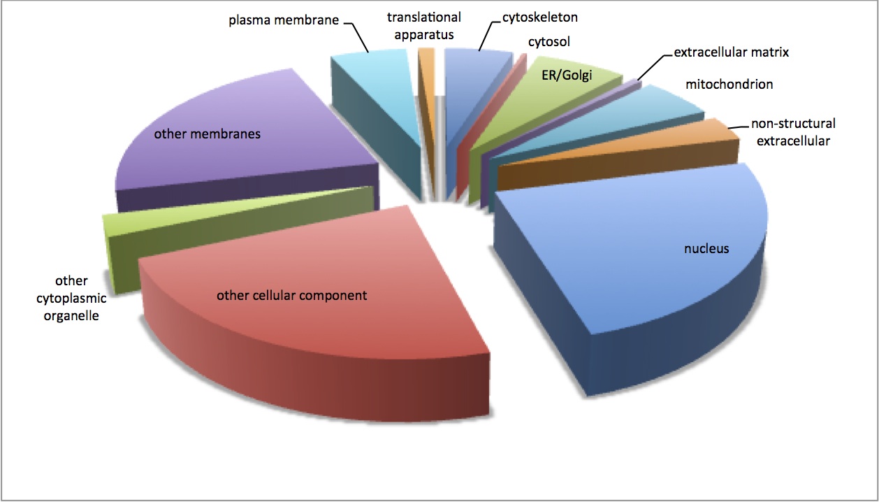
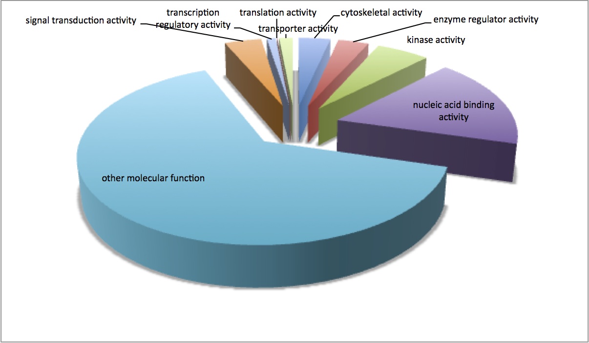
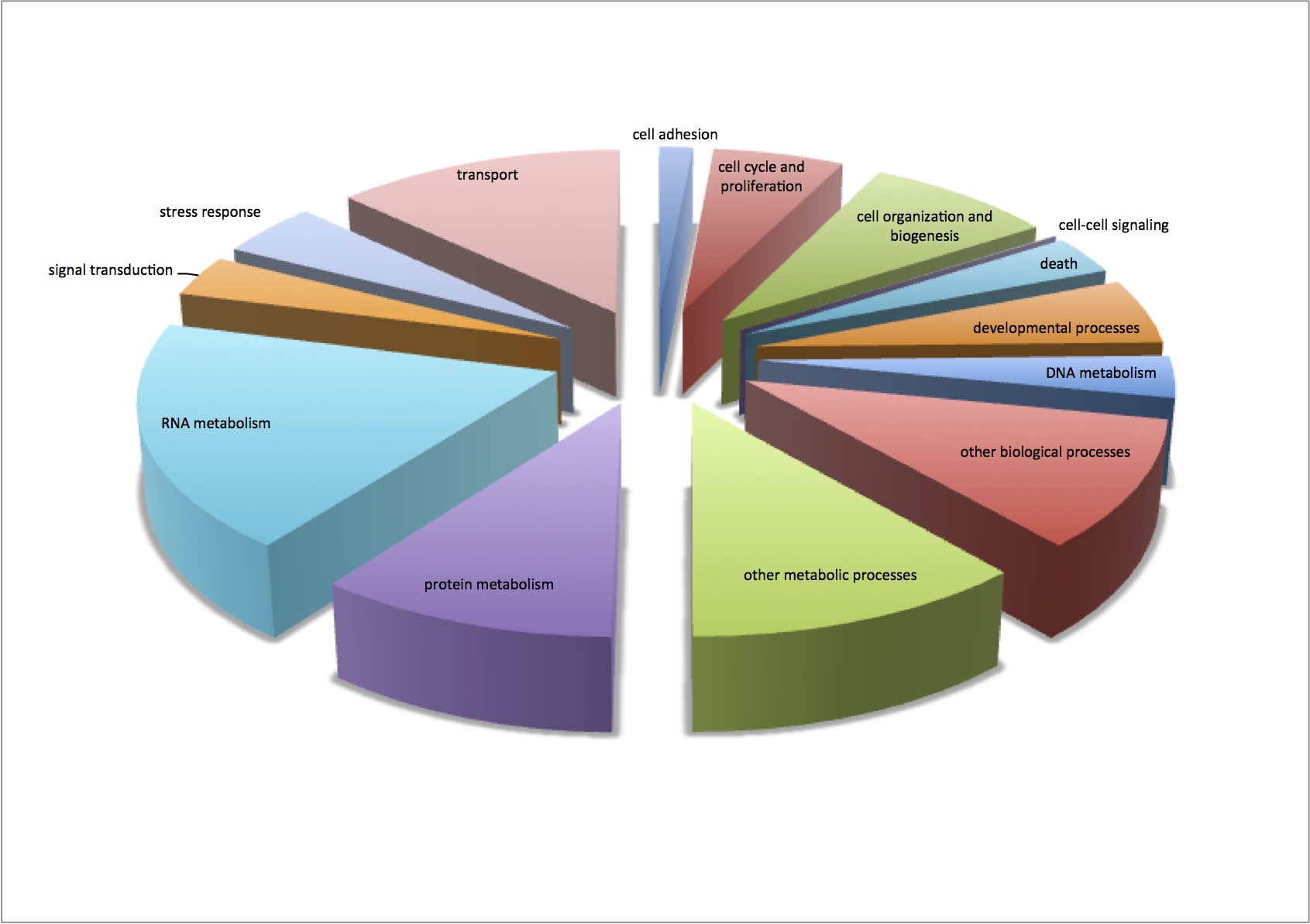
Made pie charts for the GO molecular function and cellular components (continuation of 1/9/13 analysis). Pie charts are made from non-redundant associations between contigs and GO terms based on SPID annotations. The first chart is the cellular components and the second is the molecular functions.
MeDip qPCR
MeDip qPCR of Claire's heat shocked C. gigas samples from class (methylated and unmethylated fractions, control, HS 35C, and HS 40C). See below for qPCR protocol. Exported data to qPCR miner following Mac's instructions (https://www.evernote.com/shard/s74/sh/dd4fbb95-67d2-410f-8749-51a47b76afbf/eec394e2cbad896cf383e97486efab9d).
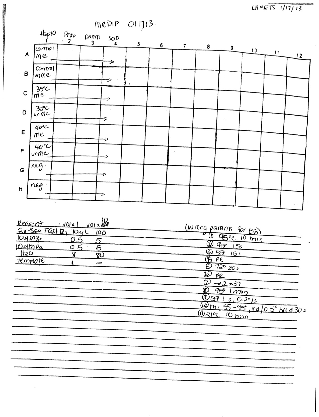
January 16, 2013
Secondary Stress: Proteomics and RNA-Seq
Created a new history in Galaxy: Cg proteomics - new GO. I am going to use the new GO and SPID files downloaded yesterday to re-annotate and analyze some of the files used for the RNA-Seq and proteomics analysis. I want to make sure my annotations are up to date for the manuscript. The gene information file that I removed the header from yesterday does not maintain the integrity of its columns when uploaded to Galaxy. I am uploading the original file from EMBL and will manipulate it in Galaxy to get the format correct.
Attempt of pathway analysis using R package CePa. Tried both methods of pathway analysis as outlined in publication (Gu & Wang 2013): gene set analysis (GSA) and over-representation analysis (ORA). For GSA, used SPID annotations to identify proteins. The data used have already been filtered to have at least 10 spec counts across replicates. If multiple proteins matched to the same SPID, the spectral counts were summed. The final spreadsheet (all protein spid expression for CePa.csv) has SPIDs as row names and individual oysters as column headers. There were no significant pathways identified for a comparison between high and low pCO2. Also did the GSA for the effect of MS Across both pCO2 treatments and the effect of MS at just ambient pCO2: there were no significant pathways. For the ORA, used the enriched gene sets identified on 12/11/12. Ran CePa for all gene sets - genes enriched at high pCO2, during MS at high pCO2, at ambient, and ambient MS. There were no significant pathways. R code can be found in my evernote (https://www.evernote.com/Home.action#b=6020fc12-578e-45b7-ae19-e768926a10c9&st=p&n=3e120664-9b18-4b4c-95aa-61214bea9010).
I'm going to re-do heat maps for transcriptomics and proteomics using only genes/proteins that contribute significantly to differentiation between treatment groups. Made a file of the proteins that are significant for the proteomics (without low abundance proteins) NMDS at the 0.05 and 0.01 levels. In Galaxy, joined this file to a file with spec counts across all biological replicates.
Secondary Stress: Fatty acids
Removed samples from freeze dryer and put lids back on. A chunk of sample 24 was lost (it looked like gill and mantle). Homogenized the freeze dried tissues with a pestle, rinsing with EtOH and nanopure water between samples (followed by drying pestle thoroughly on a clean kimwipe). Stored samples at -20C.
January 15, 2013
Bioinformatics: Assignment 1
Continuation of Part B from 1/9/13. Instead of trying to do a tblastn, will translate the database (unknown contigs from part A) and do a blastp. Uploaded fasta of contings to Galaxy. Used the emboss tool transeq to make protein sequences from the nucleotide sequences: all 6 frames, standard code (defaults for other options). Filel = transeq on unknown transcriptome 31545.fasta.
Made blast database from the translated transcriptome.
./makeblastdb -in /Users/Emma/Documents/bioinfo_assignment_1/transeq_on_unknown_transcriptome_31545.fasta -dbtype prot -out /Users/Emma/Documents/bioinfo_assignment_1/Protein_database_for_Part_B
Ran blastp of protamine sequences against protein database. Tried with e-value cutoff of 1E-5 and got 0 results. Upped e-value cut-off to 1 and got only 1 hit. With e-value cutoff of 1000 got 3 hits.
./blastp -num_threads 8 -out /Users/Emma/Documents/bioinfo_assignment_1/protamine_seq_orthologs -db /Users/Emma/Documents/bioinfo_assignment_1/Protein_database_for_Part_B -outfmt 6 -evalue 1000 -max_target_seqs 1 -query /Users/Emma/Documents/bioinfo_assignment_1/protamine_sequences.fasta.txt
Secondary Stress: Proteomics
Downloaded gene information and gene association files from EMBL (www.ebi.ac.uk/GOA/downloads.html). I will use these files to redo the GO analyses for the transcriptomics and proteomics that I plan on including in the manuscript. The gp information file gives the gene name/annotation for the swiss prot IDs. The gene association file gives the GO terms associated with each SPID. In the gp info file, there is an 18-line header that probably wouldn't mesh well with Galaxy. I can't delete it in excel or text wrangler because the file won't load completely in either application. It opens in text edit, but the app crashes every time I try to delete something. I ended up reading the file into R, skipping the first 18 lines, and then exporting it as a tab-delimited file. This is pretty inelegant because there are a number of columns that are useless (including 3 blank ones at the end of the file), but I can't figure out how to get rid of them.
gp.info<-read.table('gp_information.goa_uniprot', skip=18, sep='\t', fill=T)
write.table(gp.info, file='swissprot gene annotation 011513', sep="\t", quote=FALSE, col.names=c("UniProtKB", "Swiss-Prot", "Accession", "Gene Abbrev", "Gene name", "Gene Abbrev2", "protein", "taxon ID", " '', " '', " ''))
Secondary Stress: Fatty acids
Morgan Bond helped me set up the freeze dryer to freeze dry my oyster tissues. My original plan was to do just the digestive gland, but most of my oysters were too small to subsample the DG effectively so I am doing the whole body tissue (minus the gill which was previously sampled for transcriptomics and proteomics). For 400 uatm I am using samples 3*, 6*, 9*, 12*, 15, 18, 21, and 24 (*denotes an oyster also sequenced for proteomics). For 1000 uatm I am using samples 291, 294, 297, 300, 303, 306, 309, 312. For 2800 uatm I am using samples 219, 222*, 225*, 228*, 231*, 234, 237, and 240. Samples were kept on dry ice until they were placed in the freeze dryer. To use the freeze dryer, turn on (switch in back), put plastic cylinder on top, and then press "condense button" (this cools it down). Place the metal tray on top of the cylinder and put the rubber gasket on the lid. Place the samples on the tray (my samples are in 2 mL screw cap tubes with the lids removed) and put the lid over the tray. Press "vacuum" to bring the pressure down. Shortly after pressing "vacuum" one of the samples (24) popped out of its tube so we stopped the vacuum and put it back in. After starting up again about 6 samples started poking out of their tubes, but only one eventually came out the entire way (sample 225). Sam noted that if I had poked holes in the tube lids then the air still could have escaped but the tissue would have been trapped.
January 11, 2013
Secondary Stress: Fatty acids
Learned how to do day 2 of FA extraction (transmethylation). Set up a time next week to freeze dry samples so that they can be extracted.
January 10, 2013
Secondary Stress: Fatty acids
Learned how to do day 1 of fatty acid extraction. Protocol uploaded here (http://eagle.fish.washington.edu/oyster/FA%20protocol.pdf) and (http://eagle.fish.washington.edu/oyster/FA%20transmethylation.pdf).
Secondary Stress: Proteomics
Research into how to represent relationships among proteins in response to OA stress (i.e. pathway analysis). On the raw total counts (summed across tech reps for each oyster, at least 10 spec counts for protein to be included) made a Pearson's correlation coefficient matrix. Plotted the matrix in R using levelplot in lattice.
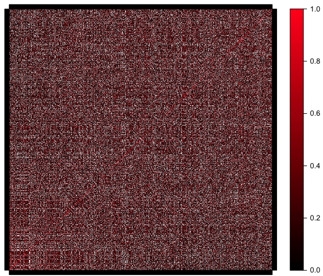
This graph isn't very easy to read and you can't see any pattern among the proteins. I've looked a bit in other papers and it seems that if pathway analysis is done, the authors use IPA. This has been done in non-model vertebrates (pied flycatchers, whitefish), but not in invertebrates. In bees, a pathway was constructed but just out of the few proteins that were highly correlated with behavioral traits of interest. I could go a similar route and try to make a pathway from the proteins that are differentially expressed due to ocean acidification and/or mechanical stress.
January 9, 2013
Bioinformatics: Assignment
Downloaded files from Eagle for parts a and b of assignment (a = http://eagle.fish.washington.edu/cnidarian/fish546/Unknown_Transcriptome_31545_contigs.fa, b = http://eagle.fish.washington.edu/cnidarian/fish546/protamine_sequences.fasta )
On Mac mini opened terminal and navigated to ncbi blast application (cd /Users/Shared/Apps/ncbi-blast-2.2.27+/bin). This is the folder where the blast applications are located.
Part A
downloaded Swiss Prot database from www.ebi.ac.uk (at the very bottom of the page, the fasta file for UniProtKB/Swiss_Prot). File is called uniprot_sprot_010913.fasta Made database of these sequences called uniprot_db_010913
./makeblastdb -in /Users/Emma/Documents/bioinfo_assignment_1/uniprot_sprot_010913.fasta -dbtype prot -out /Users/Emma/Documents/bioinfo_assignment_1/uniprot_db_010913
Successfully created database. Ran blastx of nucleotide queries against the swiss prot db.
./blastx -num_threads 8 -out /Users/Emma/Documents/bioinfo_assignment_1/blastx_output -db /Users/Emma/Documents/bioinfo_assignment_1/uniprot_db_010913 -outfmt 6 -evalue 1E-5 -max_target_seqs 1 -query /Users/Emma/Documents/bioinfo_assignment_1/Unknown_Transcriptome_31545_contigs.fa.txt
Notifications popped up in Terminal during blast: Selenocysteine (U) at position ... replaced by X.
Blastx finished. Uploaded output of blastx to Galaxy and joined with files of Swiss Prot titles, Go and GO Slim terms.
Part B
Will need to do a tblastn of the protein sequences (protamine_sequences.fasta) against a database made from the nucleotide sequences in the part A file.
Made a blast database of the nucleotide sequences using the following code:
./makeblastdb -in /Users/Emma/Documents/bioinfo_assignment_1/Unknown_Transcriptome_31545_contigs.fa.txt -dbtype nucl -out /Users/Emma/Documents/bioinfo_assingnment_1/Nucleotide_database_for_Part_B
Database was successfully created. Ran tblastn of protamine sequences against db.
./tblastn -num_threads 8 -out /Users/Emma/Documents/bioinfo_assignment_1/protamine_seq_orthologs -db /Users/Emma/Documents/bioinfo_assignment_1/Nucleotide_database_for_Part_B -outfmt 6 -evalue 1E-5 -max_target_seqs 1 -query /Users/Emma/Documents/bioinfo_assignment_1/protamine_sequences.fasta.txt
This didn't work, error = Warning: could not calculate ungapped Karlin-Altschul parameters due to an invalid query sequence or its translation. Please verify query sequence(s) and/or filtering options.
The query sequences are very short protein sequences that are highly repetitive. I blasted one manually (pblast against swissprot) and it did return the correct sequence in genbank. I then used tblastn (against nucleotide collection) and got the same error from genbank that I got from the terminal-based blast. I did tblastn of the sequence against ref seq and got the error once again.
Secondary Stress: Proteomics
Continuation of analysis of combined QE and OT data
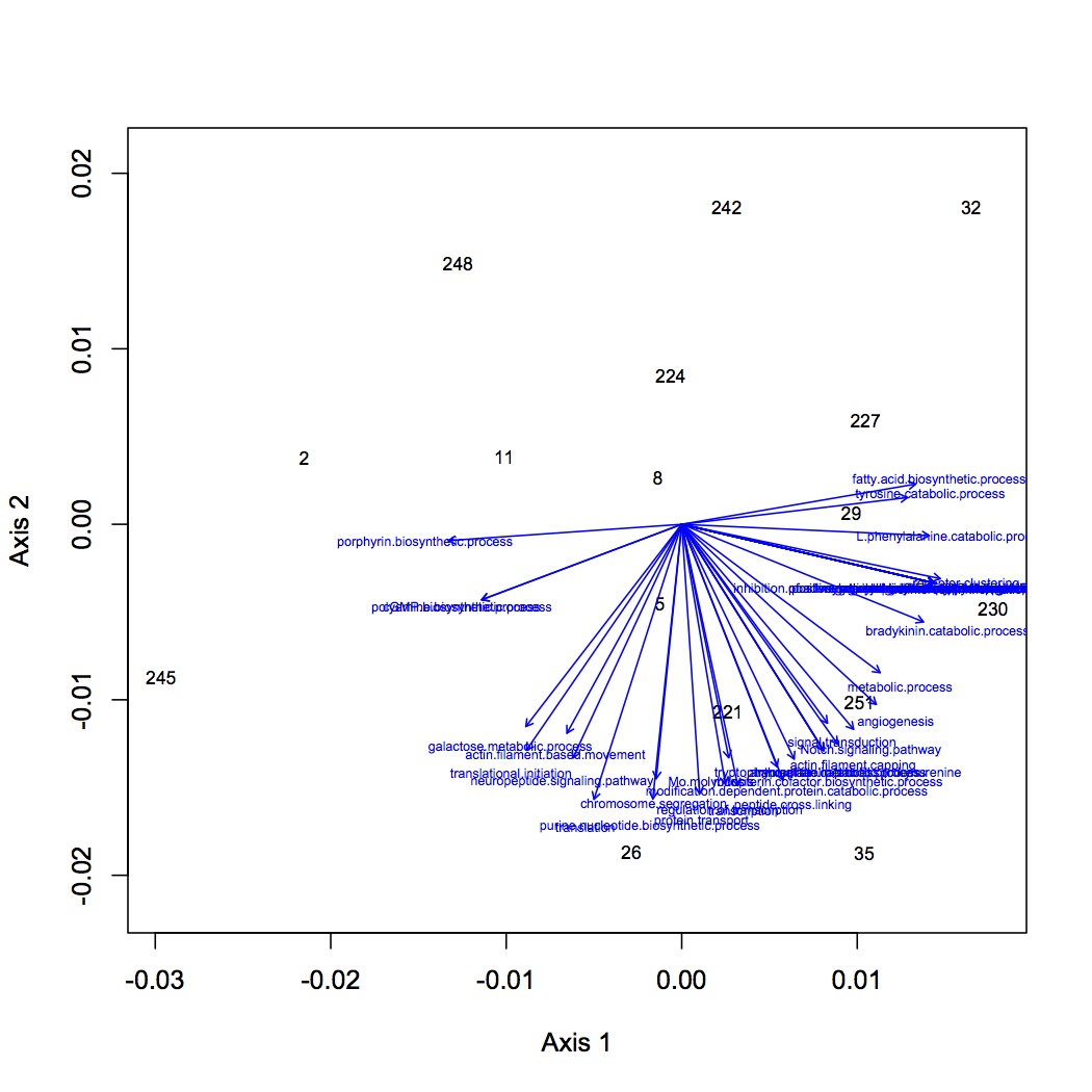
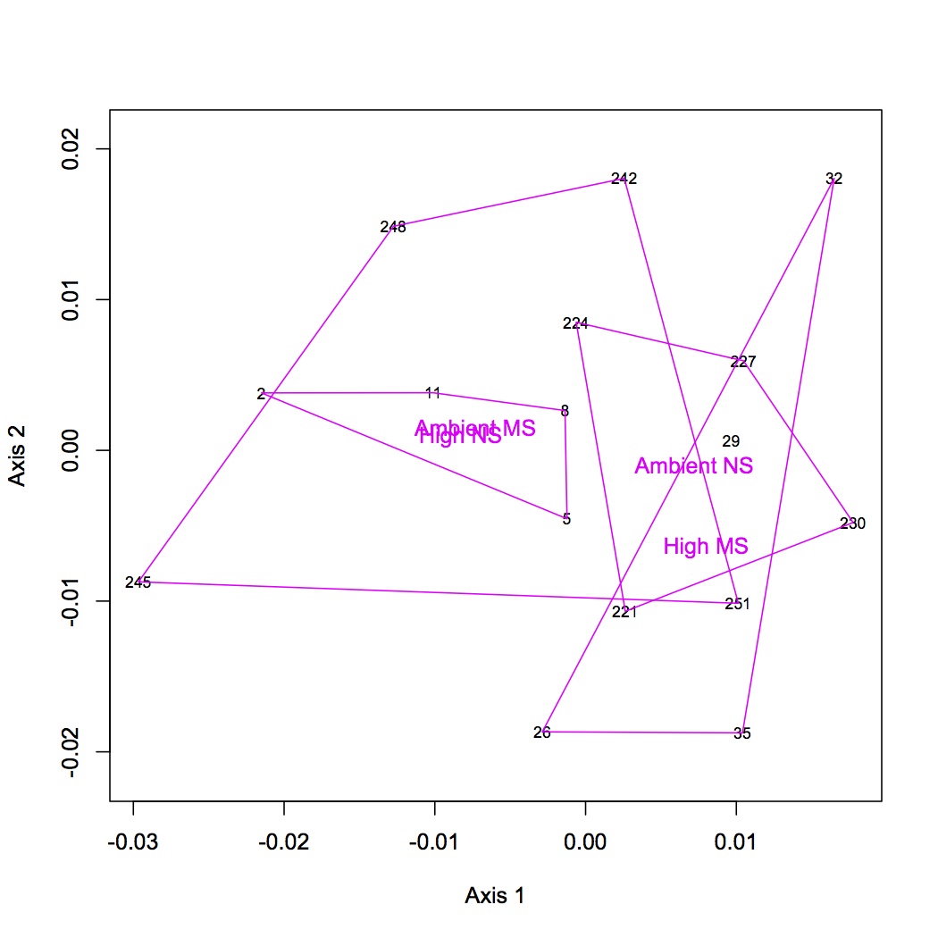
From the file created yesterday, summed spec counts for each oyster within GO categories. This produces an input file for multivariate stats in R. Did NMDS and ANOSIM of the GO data (see NMDS with loadings at alpha less than 0.01 and with polygons below). ANOSIM resulted in no significant difference due to treatment (either single effect of pCO2 or MS or combined effects of both).
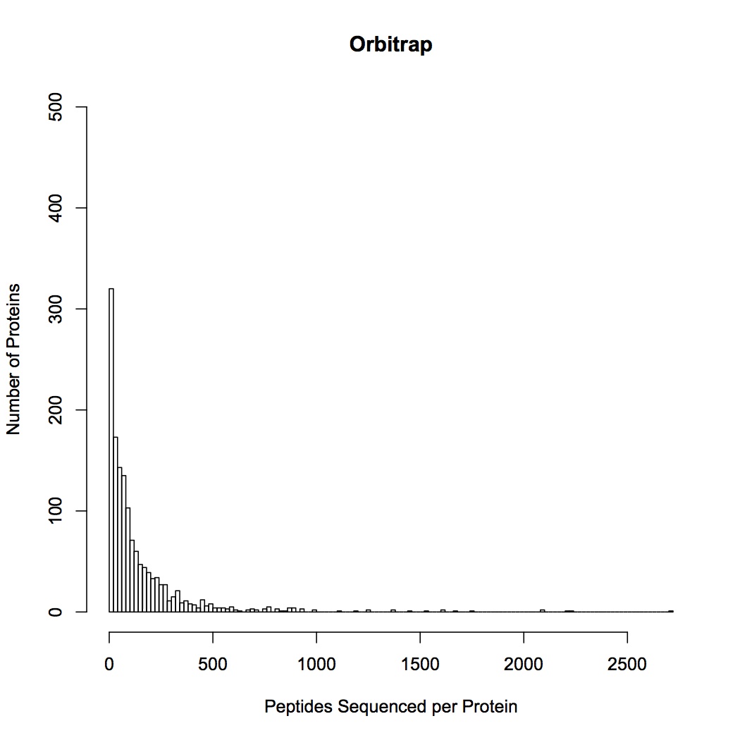
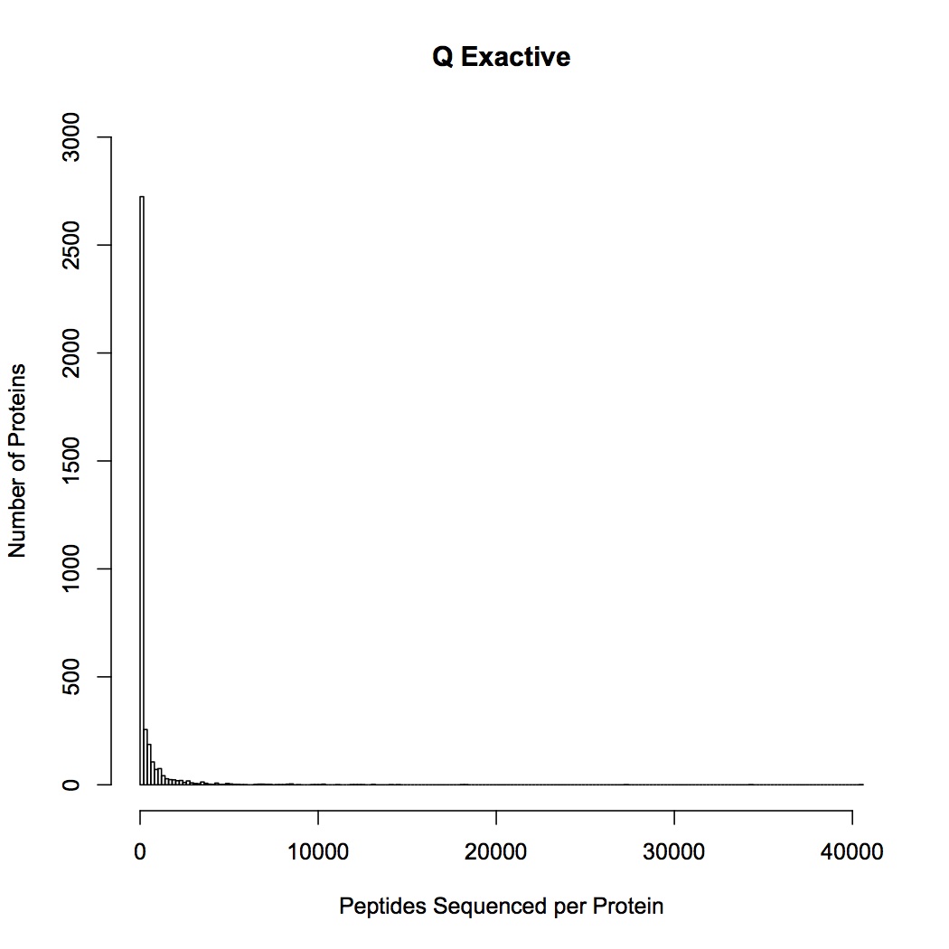
Comparison of QE and OT sequencing - made histograms of the number of proteins sequenced for groupings of number of peptides sequenced (i.e. frequency of proteins identified by 1 sequenced peptide, by 2 peptides, etc.). QE sequenced more peptides by far, but the large majority of them are low frequency proteins, whereas OT seemed to get proteins at many different frequencies. This may be part of the problem as to why the OT data are significant for differential response to treatments and QE are not (there is a lot more "noise" of low frequency proteins in the QE data).
January 8, 2013
Secondary Stress: Proteomics
Analysis of combined QE and OT data
Made a file of proteins that were sequenced by both platforms and uploaded to Galaxy (4,296 proteins). This file has been filtered to remove redundancies. To this combined proteome joined files of spec counts for QE and OT data.
Created a worksheet for just the total spec counts for each protein across replicates on both QE and OT. In cells that contained ".", replaced with a 0. Removed proteins that had fewer than 10 spec counts across all replicates on both platforms (n=1792).
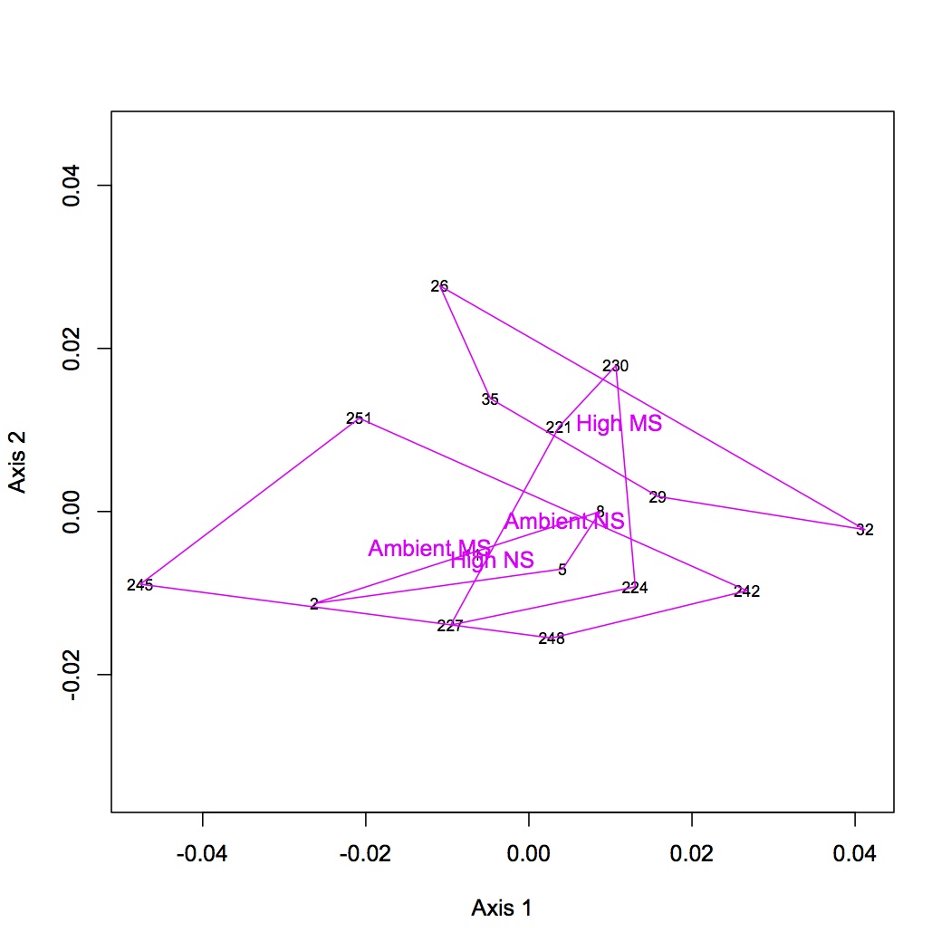
Summed spec counts across platforms for each oyster. Using Bray-Curtis dissimilarity did NMDS and ANOSIM in R. (Did the same analyses for all proteins together and for dataset of removed low abundance proteins - expressed in fewer than 8 oysters. The results were similar for both and the NMDS below is for the entire protein dataset.) There was no significant different when considering only pCO2, only MS, or combined pCO2 + MS.
Uploaded file of summed spec counts to Galaxy (summed spec counts for annotation). This file includes only proteins that have at least 10 spectral hits across replicates and platforms. Annotated file with SPIDs, GO, and GO Slim terms. At this time I will focus only on the annotations that correspond to GO biological processes. Created separate worksheets with the CG ID, columns for the total spec counts for each oyster, and either the corresponding GO or GO Slim term. Removed redundancies. Next step is to sum the spec counts within GO or GO Slim categories to make input file for NMDS.
January 7, 2013
Secondary Stress: Proteomics
QE mzXML files are downloaded to eagle. Moved xml files to the same folder on eagle (only moved the v9 interact files, those that were searched against the oyster genome and have been filtered for high probability peptides).
Set up Skyline as described 12/11/12. Library made of v9 peptides is called "QE proteins".
I can't get Skyline to work with the QE data. I'm going to abandon this avenue for now and move on to analysis of the combined dataset. It seems like there might be some information on the Skyline support forum if I want to continue later.
Secondary Stress: RNA-Seq
Continuation of analysis from 1/4/13
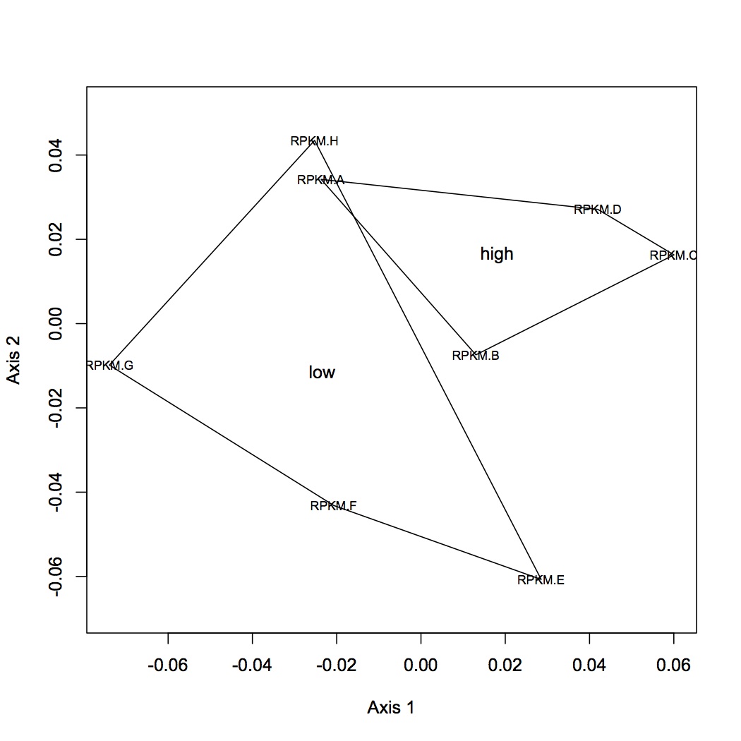
Did cluster analysis and NMDS on RPKM dataset with low abundance transcripts dropped (transcripts must be expressed in a minimum of 4 oysters to be included in analysis).
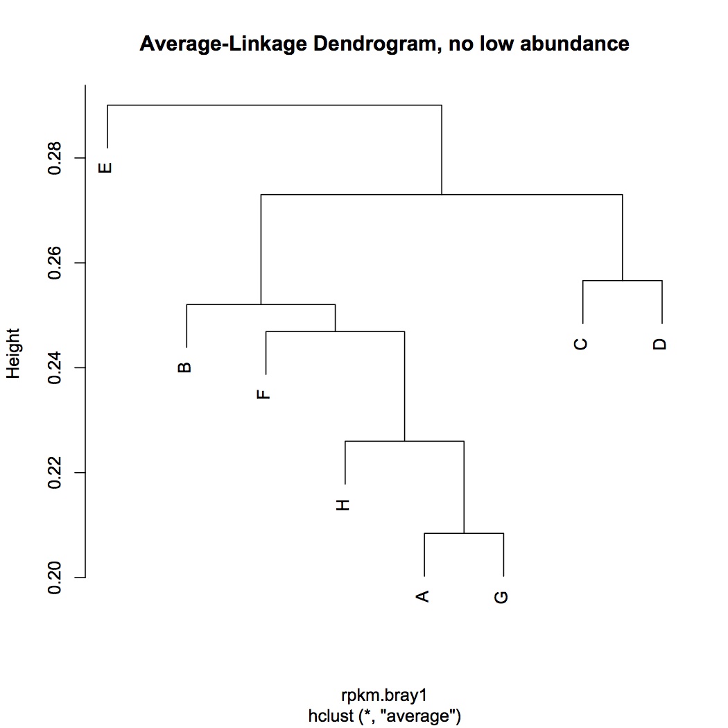
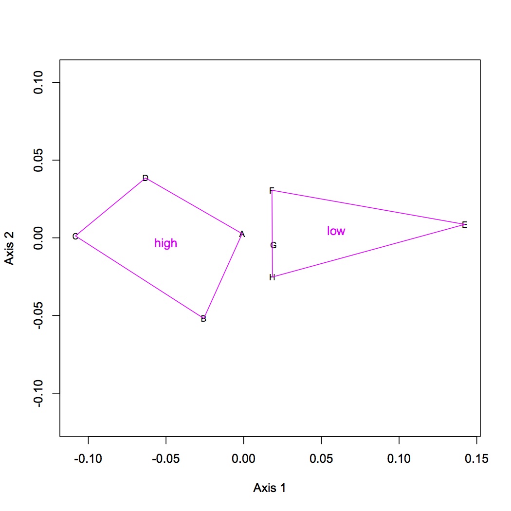
Did ANOSIM on NMDS from 1/4/13 and from today - neither showed a significant difference between treatments. Based on the NMDS, this doesn't really make sense....Need to revisit this analysis.
January 4, 2013
Secondary Stress: RNA-Seq
Analysis of RNA-Seq data (targeted 3') using RPKM instead of total reads mapped. RPKM corrects for transcript length and is a more "correct" measure of expression than total reads per gene. See 12/13/12 for description of the files used in this analysis. I'm going to basically repeat the statistics I did on the total reads of these files and use RPKM instead.
I made one document that has all of the RPKM values per oyster (n=8) for each contig (n=115999). Document is called "joined RPKM.xlsx". Removed contigs that had total RPKM across all oysters = 0 (n=3284). Ran DESeq analysis in R (first had to round down all RPKM values in Excel to nearest integer). There were 38 differentially expressed genes between low and high pCO2 with an adjusted pvalue of <0.1 (see graphs below).
Variance Dispersion
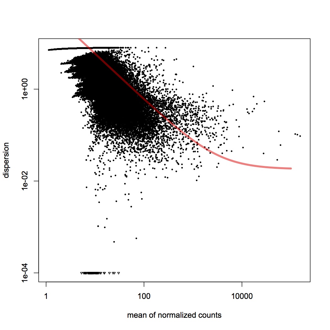
Differentially expressed genes are in red
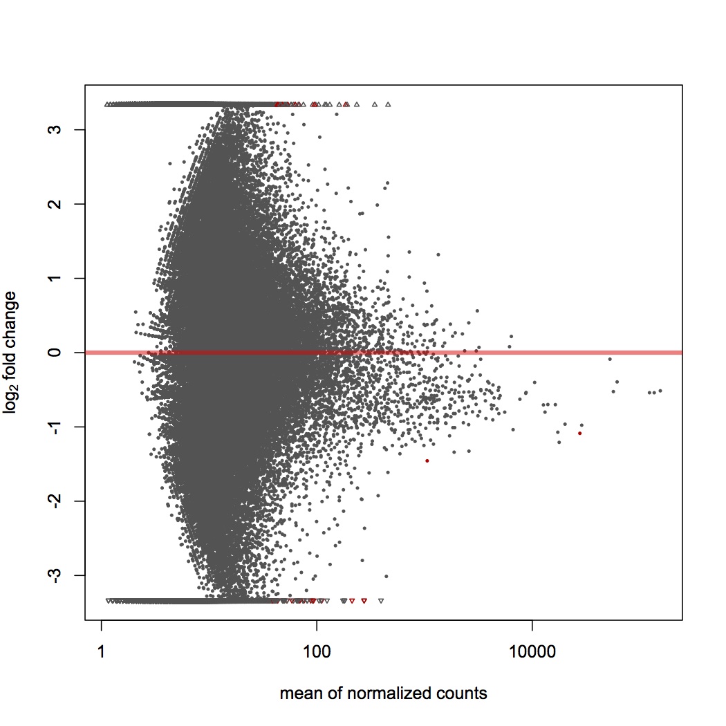
Distribution of p-values for genes
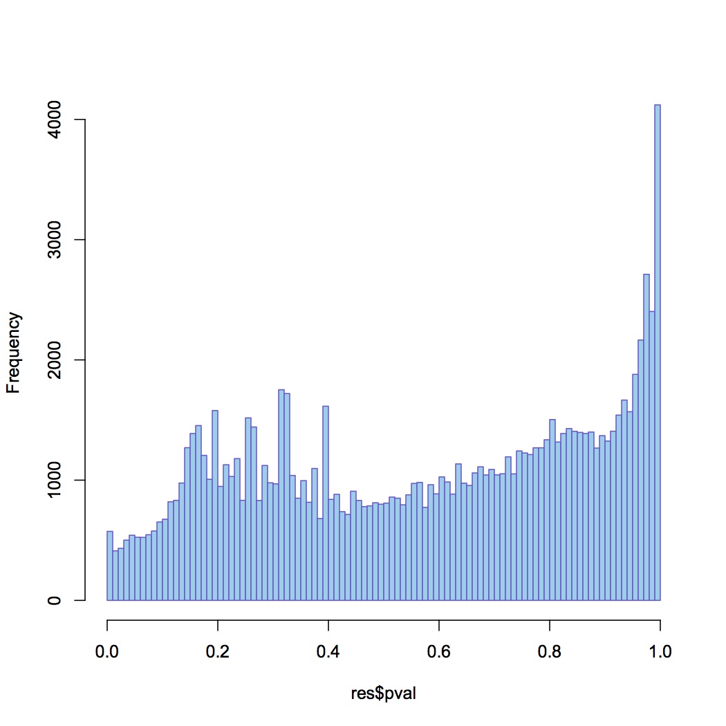
Uploaded list of differentially expressed genes to Galaxy to join with file of contig blast results (against Sigenae v8). Then joined this file with the SwissProt best hits for Sigenae contigs and with GO and GO Slim terms. Not all of the genes are annotated with Swissprot IDs and gene annotations. 15 transcripts are "down-regulated" (expressed at a lower level) at high pCO2, 23 are "up-regulated" at high pCO2. Included in the set of down-regulated transcripts are mannose receptor, techylectin (involved in innate immunity,http://www.uniprot.org/uniprot/Q9U8W7), interaptin (involved in cytoskeleton structure, http://www.uniprot.org/uniprot/O76329), lectoxin (this is expressed in the snake venom gland so it probably has a different function in the oyster..., http://www.uniprot.org/uniprot/A7X3Z0), NUF1 (essential to mitosis, http://www.uniprot.org/uniprot/P32380). Included in the set of up-regulated transcripts are hsp70 (http://www.uniprot.org/uniprot/O43301), serine/threonine protein (involved in catalytic activity, http://www.uniprot.org/uniprot/Q14738), GH21710 (http://www.uniprot.org/uniprot/B4J675), metallothionein (http://www.uniprot.org/uniprot/P23038), smc domain protein (structural maintenance of chromosomes).
hierarchical clustering of transcriptomic data
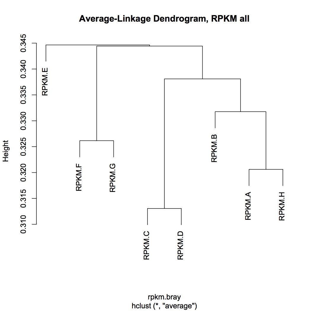
NMDS using bray-curtis
